Chapter 11 DLP and TLP¶

DLP（Data-Level Parallelism）利用同一操作在大量数据元素上的重复性，例如向量运算、矩阵计算、图像和声音处理。TLP（Thread-Level Parallelism）则把并行性提升到线程/任务层面，由软件系统或程序员识别多个可并发执行的线程。

Flynn 分类回顾

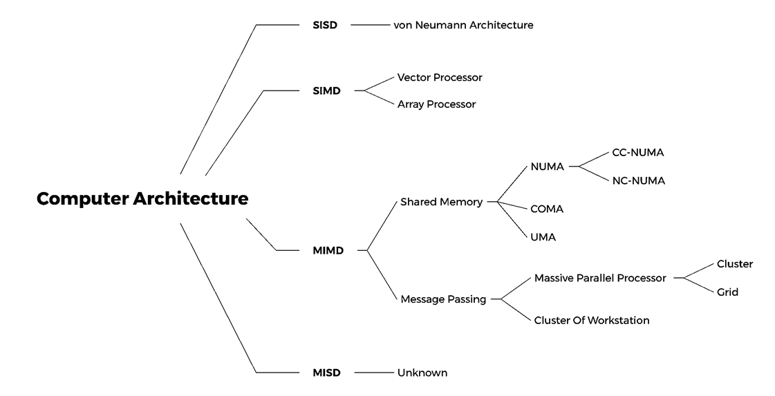
类型	指令流	数据流	典型含义
SISD	单	单	传统顺序标量处理器
SIMD	单	多	向量处理器、阵列处理机、GPU 中的 SIMD/SIMT
MISD	多	单	较少直接使用
MIMD	多	多	多处理器、多计算机、集群

DLP vs TLP

DLP：一条指令作用于多个数据元素，重点是数据并行。
TLP：多个线程拥有各自的控制流，通常意味着多个 program counters。
因此，TLP 主要通过 MIMD 结构实现，而 DLP 常通过 SIMD 结构实现。

1 SIMD: Vector Processor¶

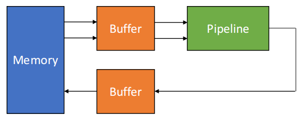
向量处理器（Vector Processor）：设置了向量数据表示和对应向量指令的流水线处理器。
标量处理器（Scalar Processor）：没有向量数据表示和向量指令的流水线处理器。

向量流水线的特点是同一向量内的元素在运算时通常很少相互相关，因此适合流水线化处理。但如果向量处理方式选择不当，也会引入数据相关和频繁的功能部件切换。

1. 1 Vector Processing Methods¶

以 \(D = A \times (B + C)\) 为例，其中 \(A\)、\(B\)、\(C\)、\(D\) 都是长度为 \(N\) 的向量。

处理方式	做法	数据相关（次）	功能切换（次）	适用性
Horizontal processing	按元素逐行计算：先算 \(d_1\)，再算 \(d_2\)，直到 \(d_N\)	\(N\)	\(2N\)	不适合向量处理器
Vertical processing	先整体计算 \(K = B + C\)，再整体计算 \(D = A × K\)	\(1\)	\(2\)	需要 memory-memory 结构
Grouping processing	把长向量分组，每组内部按 vertical 方式处理	\(S + 1\)	\(2(S + 1)\)	适合 register-register 结构

Horizontal processing 的问题

对每个分量都执行：

\[ k_i \leftarrow b_i + c_i,\quad d_i \leftarrow a_i \times k_i \]

每个元素内部存在 RAW 相关，流水线效率低。如果使用静态多功能流水线，功能部件还要频繁切换，吞吐率可能低于顺序串行执行。

Vertical processing 的适用性

Vertical processing 的源向量、目的向量和中间结果通常都放在内存中，因此要求处理器支持 memory-memory structure，典型如 STAR-100、CYBER-205。

Vertical and horizontal / grouping processing 的适用性

Vertical and horizontal / grouping processing 把向量长度写作：

\[ N = S \times n + r \]

其中 \(S\) 是完整分组数量，\(n\) 是每组长度，\(r\) 是余数。若余数也作为一组处理，则一共 \(S + 1\) 组。

计算过程

\(d_{1\sim n} \leftarrow a_{1\sim n} \times (b_{1\sim n} + c_{1\sim n})\)
\(d_{(n+1)\sim 2n} \leftarrow a_{(n+1)\sim 2n} \times (b_{(n+1)\sim 2n} + c_{(n+1)\sim 2n})\)
\(\dots\)
\(d_{(s*n+1)\sim N} \leftarrow a_{(s*n+1)\sim N} \times (b_{(s*n+1)\sim N} + c_{(s*n+1)\sim N})\)

该方式要求设置可快速访问的向量寄存器（vector registers）保存源向量、目的向量和中间结果，形成 register-register operation pipeline。典型 register-register 向量处理器包括 CRAY-1、YH-1、GRAP-3、Earth Simulator 等。

1. 2 CRAY-1¶

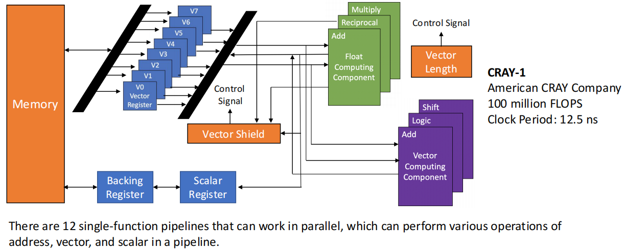
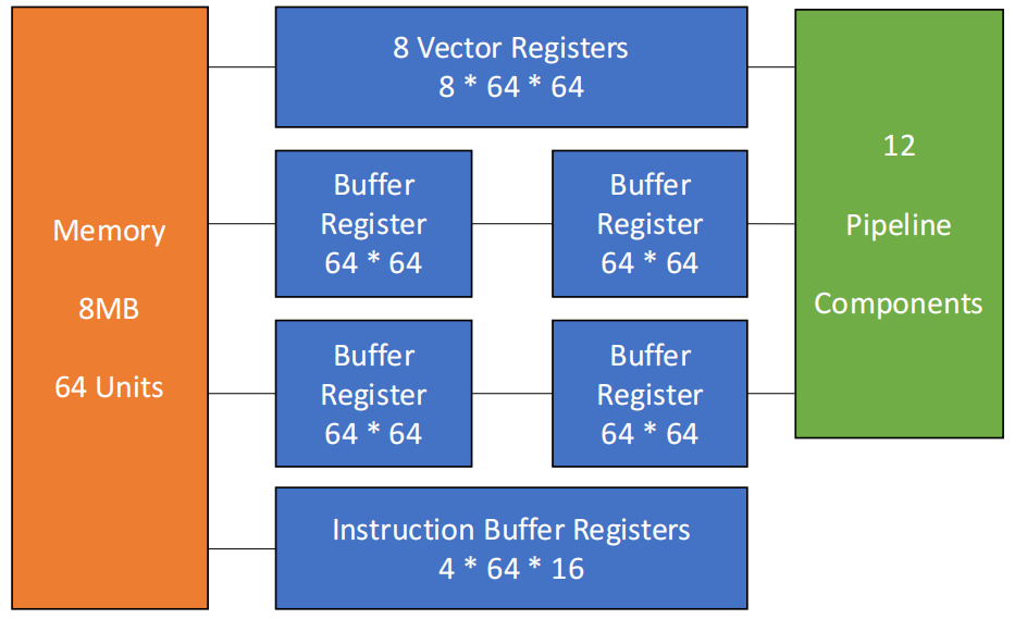
每个向量寄存器 Vi 有独立总线连接到 6 个 vector functional units
每个 vector functional unit 也有结果返回总线连接到 vector register bus

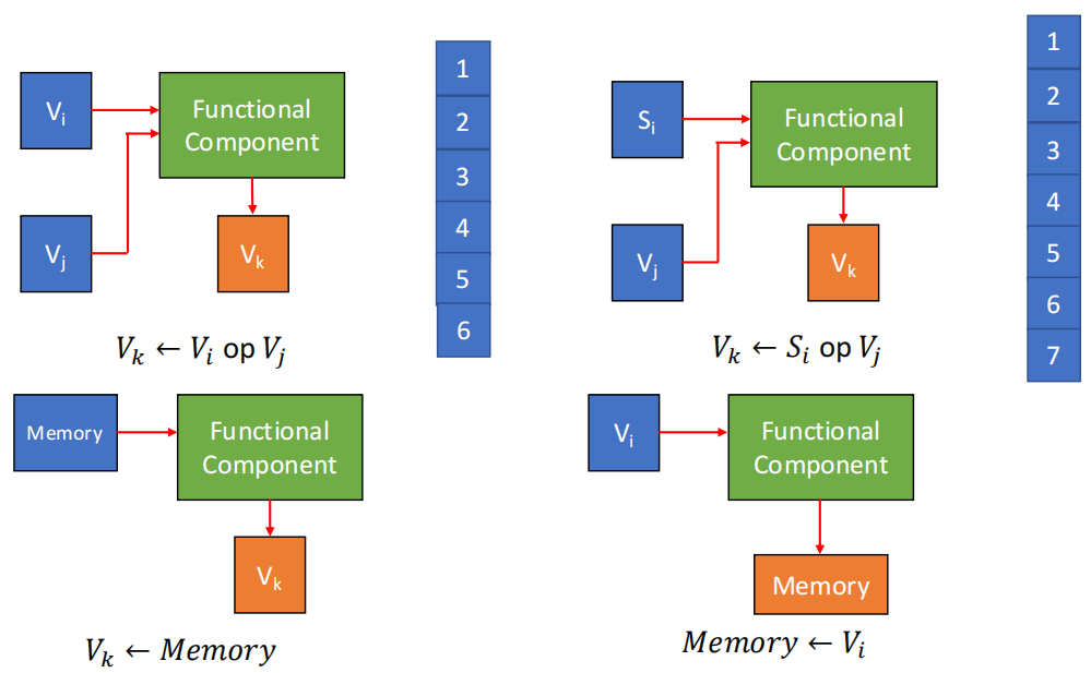
只要不存在 Vi conflict 和 functional conflict，多个向量寄存器与多个功能部件就可以并行工作。

冲突类型	含义	示例
Vi conflict	并行执行的向量指令使用同一个源向量或结果向量寄存器	\(·\) `V0 <- V1 + V2` 与 `V3 <- V0 × V4` \(·\) `V0 <- V1 + V2` 与 `V3 <- V1 × V4`
Functional conflict	并行执行的向量指令需要同一个功能部件	`V3 <- V1 × V2` 与 `V5 <- V4 × V6`

1. 3 Improving Vector Processor Performance¶

设置多个 functional units，使它们并行且各自流水化工作。

示例

CRAY-1 有 4 组 12 个 single-function pipeline components：

组件组	功能
Vector components	vector addition、shift、logic operation
Floating point components	floating add、multiplication、reciprocal
Scalar components	scalar add、shift、logic operation、number `1` / count
Address calculation components	integer add、multiplication

使用 vector chaining，加速一串有生产者-消费者关系的向量指令。

Vector chaining（向量链接）

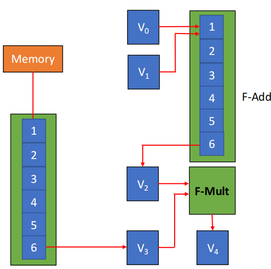
若两条向量指令存在写后读关系，且没有功能部件冲突和源向量冲突，则前一条指令产生的元素结果可以直接送入后一条指令的功能部件，让多个功能部件串接成流水线。

例题：D = A * (B + C)

假设向量长度 \(N = 64\)，B 和 C 已经在 V0、V1 中，用 3 条向量指令完成：

V3 <- A          // access vector A
V2 <- V0 + V1    // Vector B and Vector C perform floating point addition
V4 <- V2 * V3    // Floating point multiplication, the result is stored in V4

其中 V3 <- A 和 V2 <- V0 + V1 无冲突可并行，V4 <- V2 * V3 对前两条有 RAW 相关，但可以通过 chaining 边产生边消费。

假设取数、送入功能部件、写回向量寄存器各有固定启动开销，则执行时间为：

三条指令串行执行：

\[ [(1+6+1)+N-1] + [(1+6+1)+N-1] + [(1+7+1)+N-1] = 3N + 22 \]

(1) 和 (2) 并行，之后执行 (3)：

\[ max\{[(1+6+1)+N-1], [(1+6+1)+N-1]\} + [(1+7+1)+N-1] = 2N + 15 \]

使用 vector chaining：

\[ max\{(1+6+1), (1+6+1)\} + (1+7+1)+N-1 = N + 16 \]

使用 segmented vector 处理长度超过向量寄存器容量的长向量，把长向量划分为固定长度的若干 segment，每次循环处理一个 segment。该机制由硬件和软件共同控制，对程序员透明。
使用多处理器系统进一步提高性能。

示例

CRAY-2：内置 4 个向量处理器，浮点运算峰值速度最高可达 1800 MFLOPS。
CRAY Y-MP、CRAY C90：最多可搭载 16 个向量处理器。

1. 4 RV64V¶

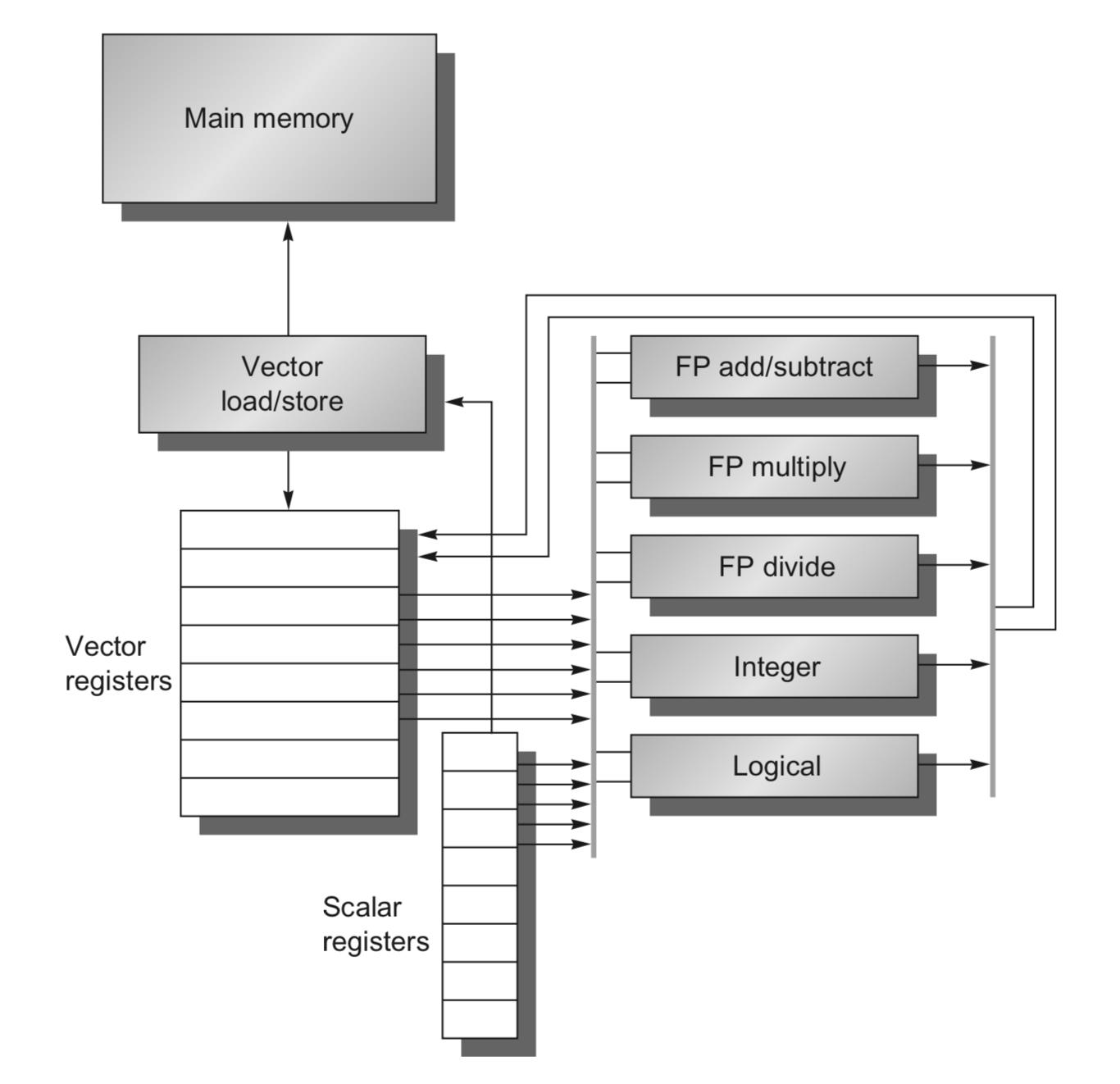
RV64V 的设计思路大体借鉴 Cray-1：

包含 32 个 64 位向量寄存器，寄存器堆配置为 16 个读端口和 8 个写端口
向量运算功能单元为全流水线设计，可检测数据冒险与控制冒险
向量访存加载 / 存储单元为全流水线设计，完成初始延迟后，每个时钟周期吞吐一个字数据
标量寄存器组包含 31 个通用整数寄存器和 32 个浮点寄存器

Example: DAXPY (Double Precision a*X plus Y)

普通 RISC-V 标量实现（一次只算 1 个元素）

fld     f0,a            # 加载标量常数 a 到浮点寄存器 f0
addi    x28,x5,#256     # 算出数组末尾地址，作为循环终止判断值
Loop:
fld     f1,0(x5)        # 从地址 x5 读取 X[i]，放入 f1
fmul.d  f1,f1,f0        # 双精度乘法：f1 = X[i] * a
fld     f2,0(x6)        # 从地址 x6 读取 Y[i]，放入 f2
fadd.d  f2,f2,f1        # 双精度加法：f2 = Y[i] + a*X[i]
fsd     f2,0(x6)        # 把计算结果写回 Y[i]
addi    x5,x5,#8        # X 数组指针向后移动 1 个双精度数（double 占 8 字节）
addi    x6,x6,#8        # Y 数组指针同步后移 8 字节
bne     x28,x5,Loop     # 如果还没走到末尾地址，跳回 Loop 继续算下一个元素

RV64V 向量版（一次批量算多个元素）

vsetdcfg  4*FP64        # 向量配置：设置向量长度，单次可处理 4 个双精度浮点数
fld       f0,a          # 依然先把常数 a 加载到标量浮点寄存器 f0
vld       v0,x5         # 向量加载：一次性从 x5 地址读入 4 个 X 元素，存入向量寄存器 v0
vmul      v1,v0,f0      # 向量-标量乘法：v1 = a × v0（4 个元素同时并行相乘）
vld       v2,x6         # 向量加载：一次性读入4个Y元素，存入向量寄存器v2
vadd      v3,v1,v2      # 向量加法：v3 = v1 + v2（4 组 $aX_i+Y_i$ 并行算出）
vst       v3,x6         # 向量存储：一次性把 4 个结果写回 Y 数组对应位置
vdisable                # 关闭向量单元，退出向量模式

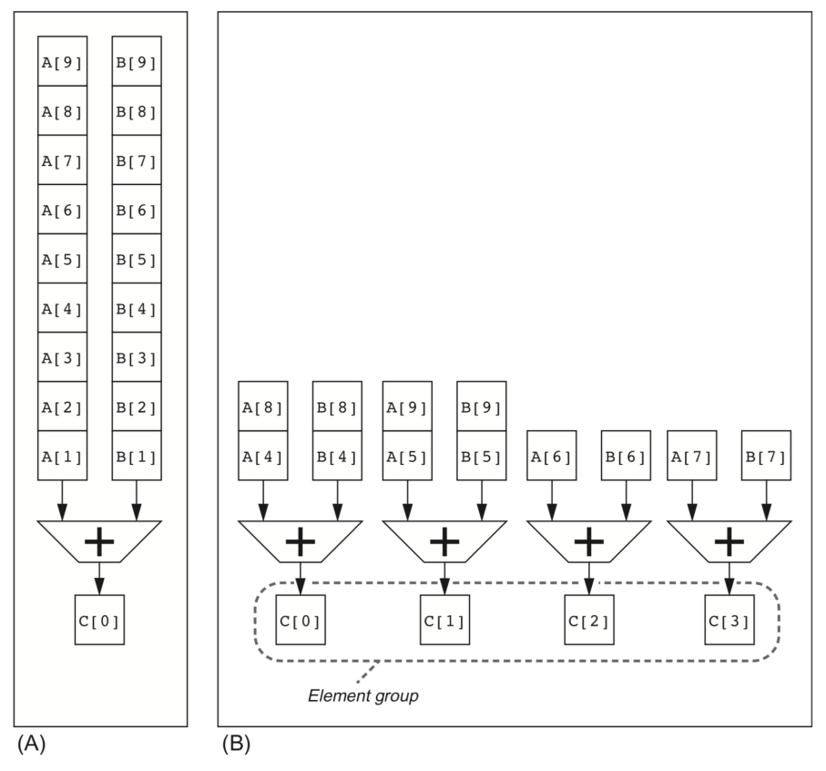
RV64V 的向量算术指令只允许向量寄存器中的第 N 个元素与其它向量寄存器中的第 N 个元素参与运算。这个性质让向量单元可被组织成多个并行 lanes，从而突破每周期一个元素的限制。

2 SIMD: Array Processor¶

阵列处理机（Array Processor） 重复设置 N 个 processing elements（PE0 到 PEN-1），通过某种互连方式组成阵列，在单一控制单元控制下，对分配到各 PE 的数据并行执行同一条指令。阵列处理机有时也称为 parallel processor。

示例：ILLIAC IV

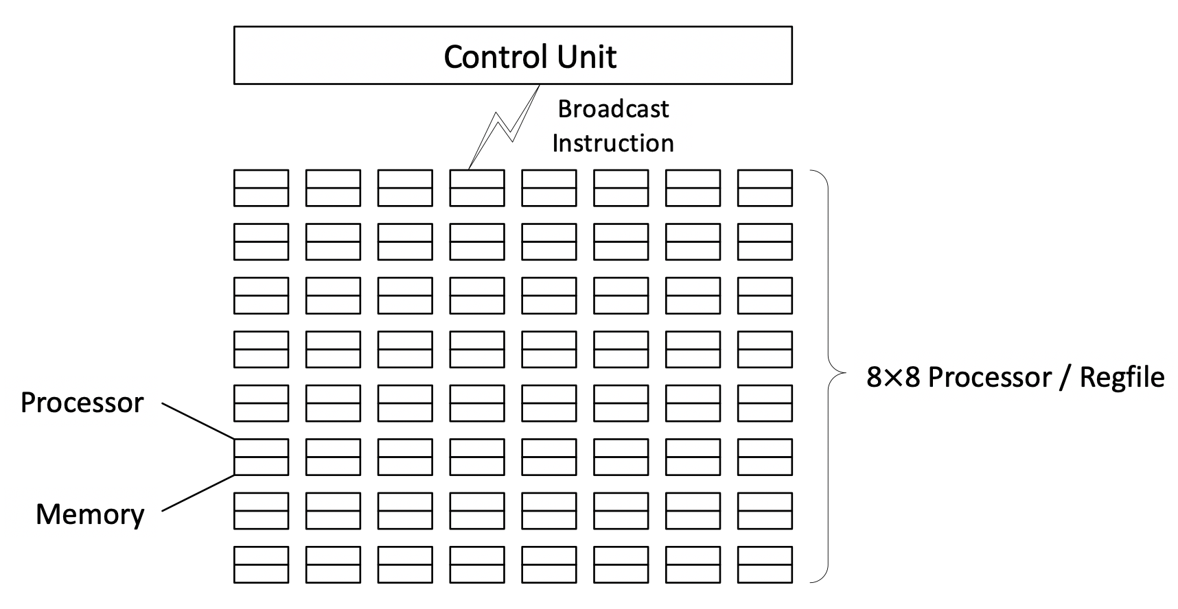
2. 1 Basic Structure¶

结构	特点
Distributed memory	每个 PE 关联自己的 memory，SIMD 阵列处理机的主流结构
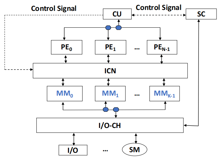
Centralized shared memory	多个 PE 通过互连网络访问集中共享 memory

Distributed memory

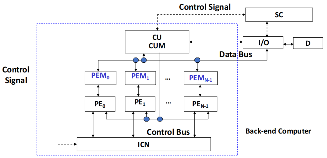
Centralized shared memory

2. 2 Interconnection Network¶

引入

如果 n 个处理单元之间都要求直接连接，则连接对数为：

\[ P = C_n^2 = \frac{n(n - 1)}{2} \]

直接路径难以实现，因此并行机通常通过互连网络（Interconnection Network）提供一步或少数几步的信息传输。

互连网络是在计算机系统内部，由 switching units 按照特定 topology 和 control mode 组成的网络，用于连接多个处理器、存储器或功能部件，通常由 5 个部分组成：

部分	含义
CPU / memory	通信端点
Interface	从 CPU/memory 获取信息并发送到另一个 CPU/memory，典型如 NIC
Link	传输数据位的物理通道，可为电缆、双绞线、光纤，支持串行/并行、半双工/全双工
Switch node	多输入多输出的信息交换与控制节点，负责 buffering 和 path selection

设计关注方面	类型
Topology	static topology、dynamic topology
Timing mode	synchronous system、asynchronous system
Exchange method	circuit switching、packet switching
Control strategy	centralized control、distributed control

网络类型	含义	示例
Static network	程序执行期间节点间连接路径固定	linear array、ring、tree、grid、hypercube
Dynamic network	由 switches 动态改变连接状态	bus、crossbar、multi-stage interconnection network

2. 3 Single-Stage Interconnection Networks¶

单级互连网络通过一个有限连接层实现任意两个处理单元间的一步或少数几步通信。

Single-stage interconnection network 的特点

结构简单，成本低
连接方式灵活，能适配算法与应用需求
传输步数少，可提高阵列运算速度
规则性和模块化较好，利于扩展
便于大规模集成

① Cube Network¶

设 \(N = 2^n\)，输入和输出端口用 \(n\) 位二进制编码：

\[ P_{n-1} \cdots P_i \cdots P_1P_0 \]

\(Cube_i\) 函数翻转第 \(i\) 位：

\[ Cube_i(P_{n-1}\cdots P_i \cdots P_0) = P_{n-1}\cdots \overline{P_i} \cdots P_0 \]

示例

\(\mathit{cube}_0(X_2X_1X_0) = (X_2X_1\overline{X_0})\)

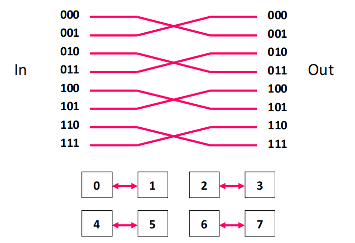
\(\mathit{cube}_0(X_2X_1X_0) = (X_2\overline{X_1}X_0)\)

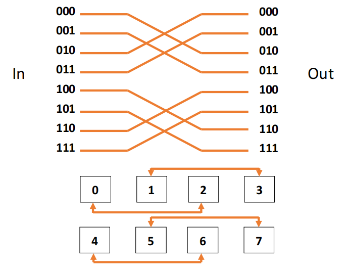
\(\mathit{cube}_0(X_2X_1X_0) = (\overline{X_2}X_1X_0)\)

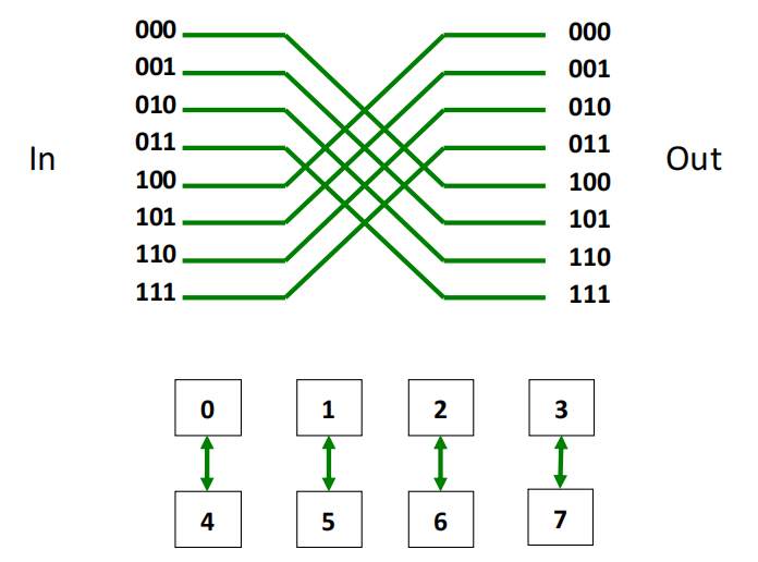
当 \(n > 3\) 时称为 hypercube network。单级 \(n\) 维 cube network 的最大距离为 \(n\)，任意两个 PE 之间最多经过 \(n\) 次传输。

② PM2I Network¶

PM2I 单级网络包含 \(2n\) 个互连函数：

\[ PM2_{+i}(j) = (j + 2^i) \bmod N \]

\[ PM2_{-i}(j) = (j - 2^i) \bmod N \]

其中：

\[ 0 \le j \le N - 1,\quad 0 \le i \le \log_2 N - 1 \]

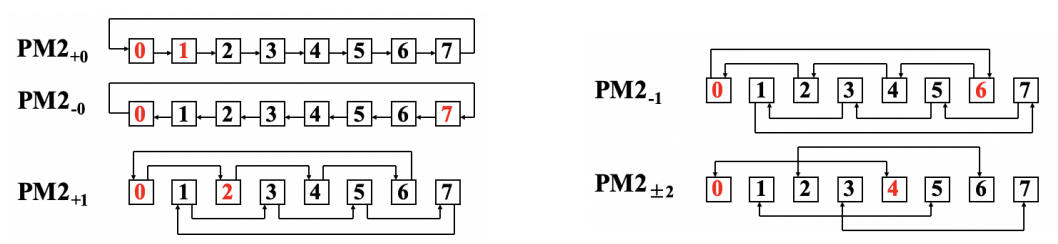
示例：\(N = 8\) 的 PM2I

- \(PM2_{+0}(j) = (j + 2^0) \bmod 8\)
\(PM2_{+0}\) / \(PM2_{-0}\) 连接相邻节点
- \(PM2_{-0}(j) = (j - 2^0) \bmod 8\)
\(PM2_{+1}\) / \(PM2_{-1}\) 连接相差 \(2\) 的节点
- \(PM2_{+1}(j) = (j + 2^1) \bmod 8\)
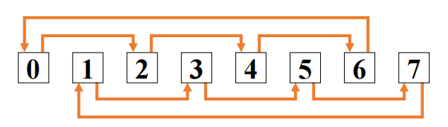
- \(PM2_{-1}(j) = (j - 2^1) \bmod 8\)
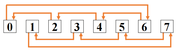
`\(PM2_{+2}\) / \(PM2_{-2}\) 连接相差 \(4\) 的节点
- \(PM2_{\pm2}(j) = (j \pm 2^2) \bmod 8\)

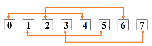
节点 \(0\) 一步可到达 \(1, 2, 4, 6, 7\)，两步可到达 \(3, 5\)。

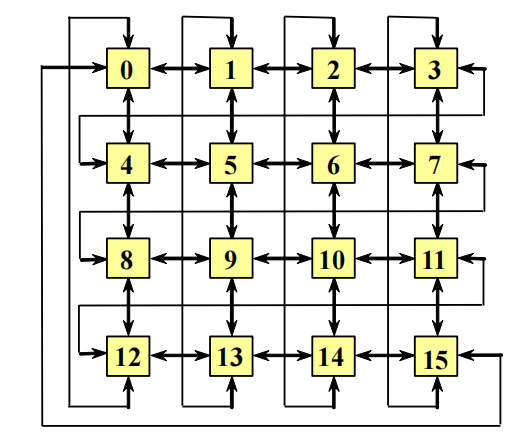
ILLIAC IV 使用 \(PM2_{±0}\) 和 \(PM2_{±n/2}\) 形成上下左右互连。

③ Shuffle Exchange Network¶

Shuffle exchange network 由 shuffle 和 exchange 两部分组成。\(N = 2^n\) 时，shuffle 函数为：

\[ shuffle(P_{n-1}P_{n-2}\cdots P_1P_0) = P_{n-2}\cdots P_1P_0P_{n-1} \]

即二进制编码循环左移一位。

示例：8 PEs

\(\mathit{shuffle}(P_2P_1P_0) = P_1P_0P_2\)

Initial Code	Before Shuffle	After 1st Shuffle	Connected PE (1st Shuffle)	After 2nd Shuffle	Connected PE (2nd Shuffle)	After 3rd Shuffle	Connected PE (3rd Shuffle)
0	000	000	0	000	0	000	0
1	001	010	2	100	4	001	1
2	010	100	4	001	1	010	2
3	011	110	6	101	5	011	3
4	100	001	1	010	2	100	4
5	101	011	3	110	6	101	5
6	110	101	5	011	3	110	6
7	111	111	7	111	7	111	7

经过 \(N\) 次 shuffle 操作后，全部 \(N\) 个 PE 恢复为初始排列顺序

从编号全 \(0\) 的节点到全 \(1\) 的节点，最多需要：

\[ n \text{ exchanges} + (n - 1) \text{ shuffles} \]

因此最大距离为：

\[ 2n - 1 \]

④ Others¶

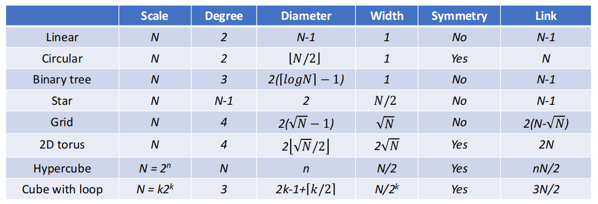
2. 4 Multi-Stage Interconnection Networks¶

动态网络

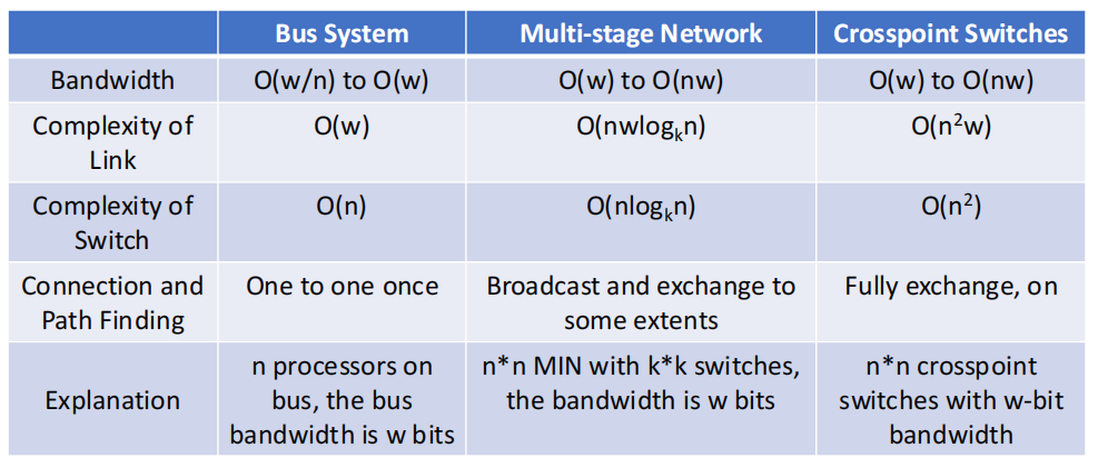
动态网络	特点
Bus	\(·\) 同一时刻只能在一对 source/destination 之间传输 \(·\) 多个请求需要 arbitration \(·\) CPU 数多时总线竞争严重，通常适合 \(<= 32\) 个 CPU
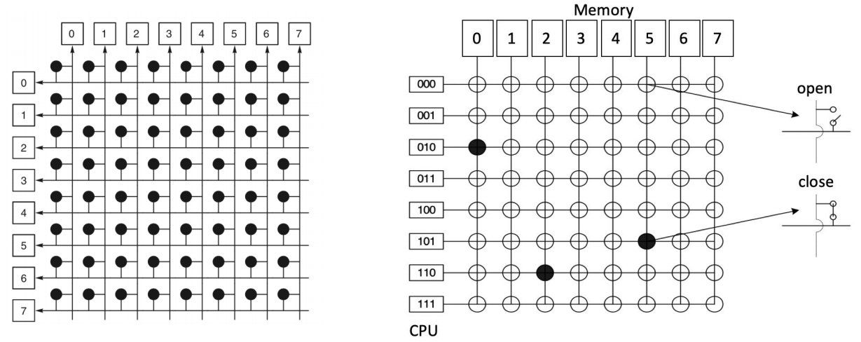
Crossbar switches	可提供完全交换能力，但硬件复杂度高
Multi-stage network	用多级小交换单元串联，在复杂度和连接能力之间折中

Linear array 与 Bus 的区别

Linear array：不同 source/destination 可并发使用系统的不同部分。
Bus：多个节点共享同一总线，时间分割使用，同一时刻只有一对节点传输。

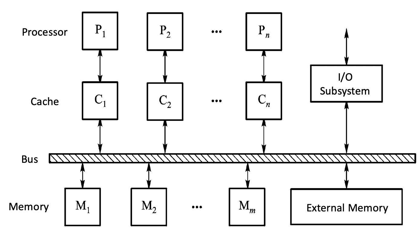
A multiprocessor system connected by bus

Crosspoint switches

拥有 \(m\) 个输入、\(m\) 个输出的开关单元记作 \(m×m\) 规格开关单元，其中 \(m=2^k\)（\(k\) 为整数），常见的规格有 \(2×2\)、\(4×4\)、\(8×8\) 等。

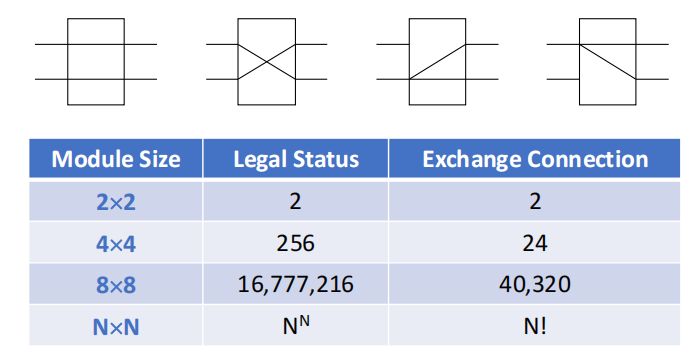
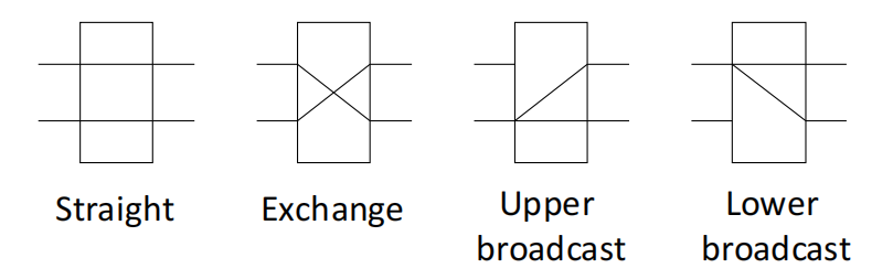
根据开关单元的功能差异，\(2×2\) 开关可分为二功能开关和四功能开关两类。

类型	支持功能	示意图
Two-function switch	straight、exchange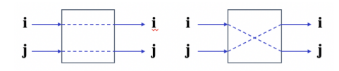
Four-function switch	straight、exchange、upper broadcast、lower broadcast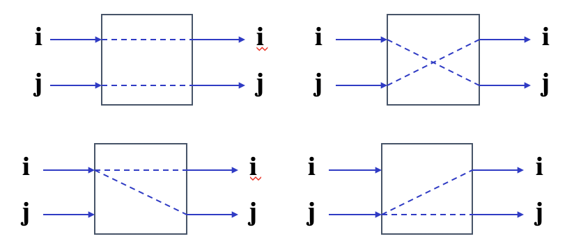

多级互连网络的差异主要来自 switch function、switch control method 和 topology。

常见 topology 包括 multi-stage cube、multi-stage shuffle exchange、multi-stage PM2I 以及上述网络的组合。

① Multi-Stage Cube Network¶

项目	内容
Switch unit	two-function switch
Control mode	stage control、part stage control、unit control
Topology	cube structure

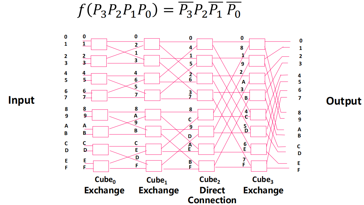
\(N\) 节点多级立方体网络拓扑图绘制步骤：

根据 \(n=\log_2 N\) 确定多级立方体网络的总级数 \(n\)
级数从输入端到输出端依次编号为 \(0, 1, \dots, n-1\)
每一级布置 \(N/2\) 个二功能交换单元
按照 \(\mathit{Cube}_i\)（第 \(i\) 维立方体置换）映射关系，对第 \(i\) 级所有交换单元的两个输入、输出端口分配编号
将相邻两级之间编号相同的交换端口相互连接

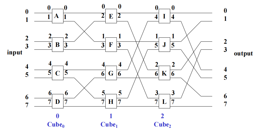
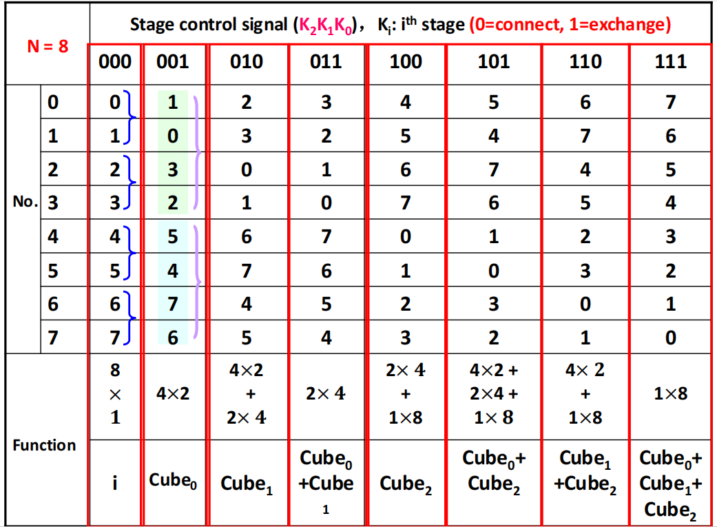
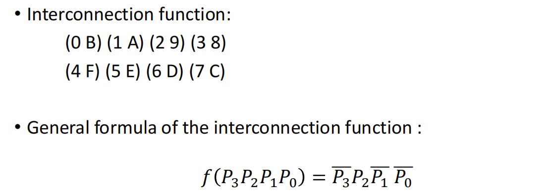
翻转网络（Flip Network）：采用级控制方式的多级立方体网络被称为交换网络，这类网络仅能实现交换函数对应的功能。
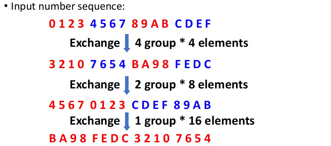
交换函数（Exchange function）：对一组元素进行对称互换操作。若某一组包含 \(2^l\) 个元素，则组内所有第 \(k\) 位元素会和该组内第 \([2^l-(k+1)]\) 位元素两两互换。

16 节点多级立方体网络实现三种对称分组交换

② Omega Network¶

\(N = 8\) Omega Network

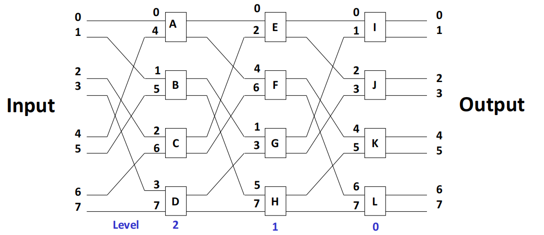
stage 数量为 \(n = log_2N\)
从输入到输出，stage 编号为 \(n - 1, ..., 1, 0\)
每级有 \(N/2\) 个 switch units
拓扑为 shuffle topology 后接 four-function switch
control mode 为 unit control

如果 Omega network 的 switching unit 只允许使用 direct connect 和 exchange，就成为 n-cube network 的 inverse network。

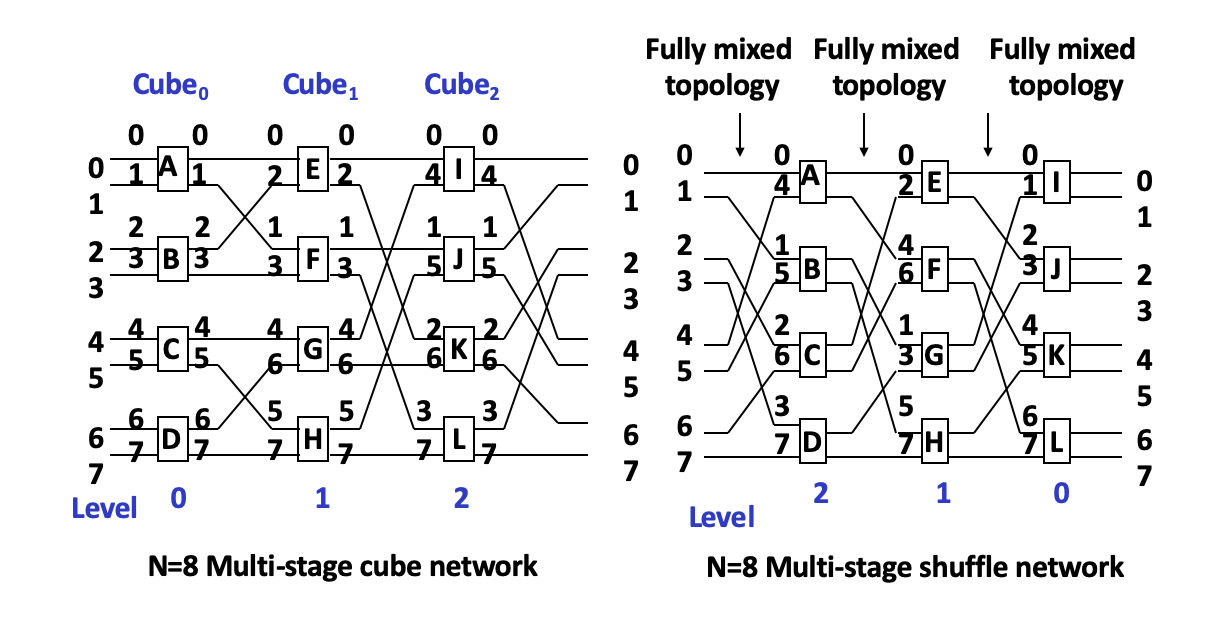
比较项	Omega network	n-cube network
Data flow level	`n - 1, n - 2, ..., 1, 0`	`0, 1, ..., n - 1`
Switch unit	four-function switch	two-function switch
Broadcast	可实现 one-to-many broadcast	不能实现

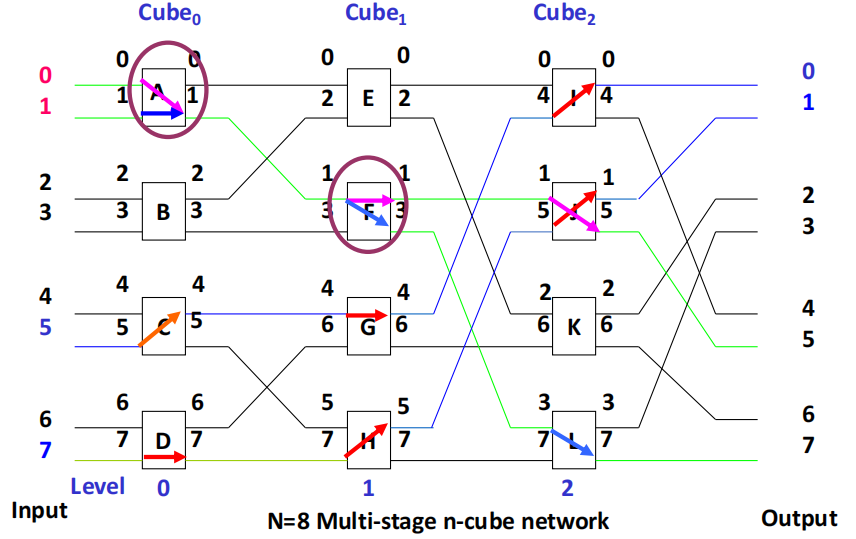
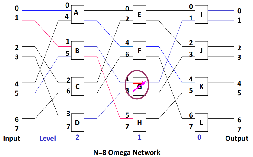
冲突路由：If the connection of 5 to 0 and 7 to 1 can be realized at the same time, can the connection of 0 to 5 and 1 to 7 be realized at the same time?

\(N=8\) 多级 n-cube：两条路径在某一级同一个交换单元内部争夺端口资源：同一个交换单元同一时刻不能同时完成两组交叉转发，出现内部冲突（路由阻塞），因此无法同时建立两条通路。

\(N=8\) Omega：两条通路到达中间级交换单元 G 时，会同时要求占用该交换单元的同一组输入 / 输出端口；一个交换单元同一时刻只能处理一组转发，无法同时满足两条路径，发生端口冲突，因此无法同时建立两条通路。

Dynamic interconnection networks 对比

Advantages of SIMD

能利用显著 DLP，尤其适合矩阵型科学计算、图像与声音等 media processing。
比 MIMD 更节能：每次数据操作只需取一条指令。
程序员仍可按较顺序的方式思考问题。

3 DLP in GPU¶

GPU 的基本思想

异构执行模型（Heterogeneous execution model）：CPU 是 host，GPU 是 device
使用 C-like programming language 编写 GPU 程序
把 GPU 的各种并行形式统一为 CUDA thread
编程模型是 SIMT（Single Instruction Multiple Thread）

CUDA（Compute Unified Device Architecture） 把 thread 作为统一抽象。执行一整个 thread block 的硬件可看作 multithreaded SIMD Processor，因此 GPU 本质上也是多线程 SIMD 处理器。

示例: DAXPY

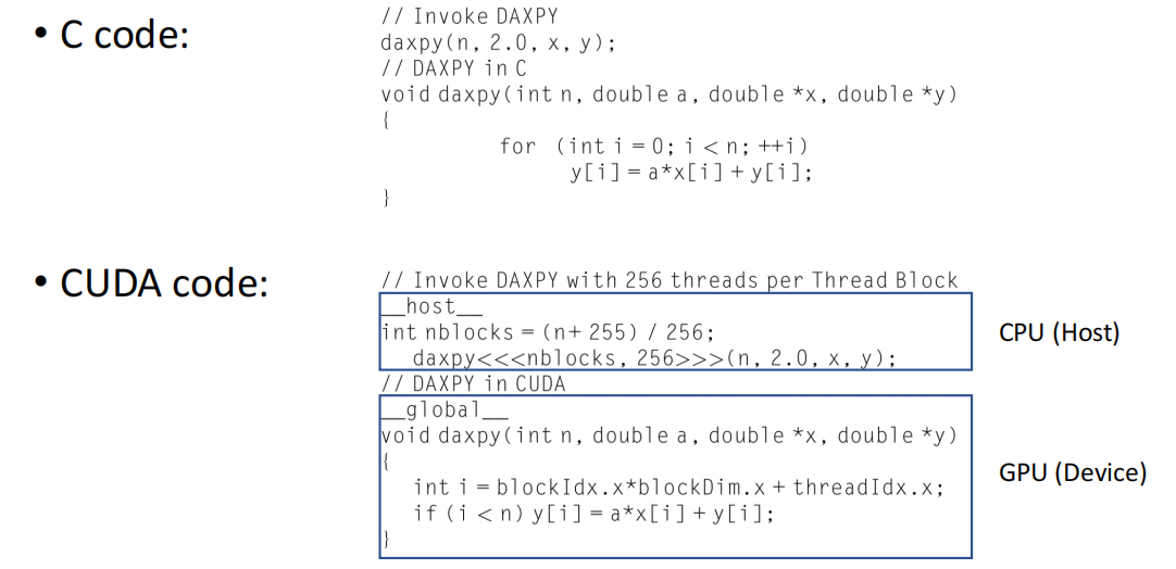
3. 1 CUDA Execution Model¶

层级	含义
Thread	通常对应一个数据元素
Thread Block	一组 threads
Grid	一组 thread blocks

GPU hardware 负责 thread management，而不是应用程序或 OS。

图示

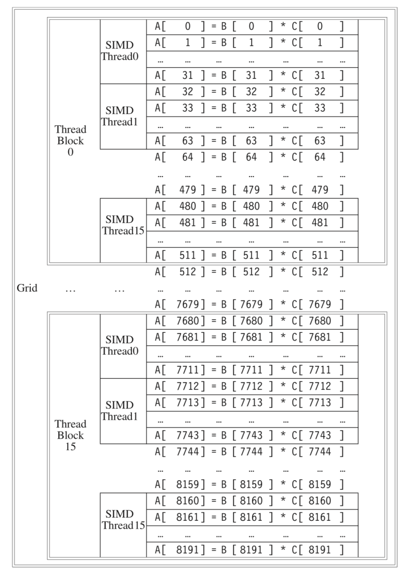
3. 2 GPU Memory Structure¶

存储结构	共享范围	类比
GPU memory	所有 grids 共享	vectorized loops 之间共享
Local memory / shared memory	同一 thread block 中 SIMD instructions 的所有 threads 共享	vectorized loop body 内共享
Private memory	单个 CUDA thread 私有	单线程私有状态

GPU 在 GPU 和 DRAM 之间加入 cache，利用 spatial locality 和 temporal locality。典型两级 cache 结构：

L1 Cache 位于 SM（Streaming Multiprocessor）内部
L2 Cache 在多个 SM 之间共享

3. 3 GPU Organization¶

GPU 组织通常可以看作：

Core -> SM (Streaming Multiprocessor) -> GPU

不同 NVIDIA GPU 架构的演进重点

架构	特点
Tesla	Core / SM / GPU 分层组织
Fermi	集成 L1 与 shared memory，SM 中 cores 更多
Kepler	巨型 SM，单个 SM 可有 192 cores
Maxwell	把 SM 拆为 4 个 blocks，调度和功耗控制更灵活，拆分 L1 和 shared memory
Pascal	L2 增大到 4MB，约为前代 7 倍
Volta	再次集成 L1 与 shared memory，instruction buffer 变为 L0 instruction cache
Ampere	L2 增大到 40MB，增加 global memory 与 shared memory 间的数据通路
Hopper	继续强化面向大规模并行和矩阵计算的组织

NVIDIA GPU 与 Vector Machine

相似点：

都适合 data-level parallel problems
都支持 scatter-gather transfers
都有 mask registers
都有 large register files

不同点：

GPU 没有传统意义上的 scalar processor
GPU 用 multithreading 隐藏 memory latency
GPU 有大量 functional units，而传统 vector processor 更像少数深流水功能部件

4 Loop-Level Parallelism¶

LLP（Loop-Level Parallelism） 关注循环迭代之间是否存在数据相关。循环往往是 DLP、TLP 和静态 ILP（如 VLIW）可挖掘并行性的来源。

判断重点是后续迭代的数据访问是否依赖前面迭代产生的值，即是否存在 loop-carried dependence。

Example 1：无 loop-carried dependence

for (i = 999; i >= 0; i = i - 1)
    x[i] = x[i] + s;

每次迭代只访问自己的 x[i]，没有跨迭代依赖。

Example 2：存在 loop-carried dependence

for (i = 0; i < 100; i = i + 1) {
    A[i + 1] = A[i] + C[i];      /* S1 */
    B[i + 1] = B[i] + A[i + 1];  /* S2 */
}

S1 在第 i + 1 次迭代会使用前一次迭代由 S1 写出的 A[i]
S2 在第 i + 1 次迭代会使用前一次迭代由 S2 写出的 B[i]
S2 在同一次迭代中还使用 S1 刚写出的 A[i+1]

Example 3：有跨迭代依赖但不是循环依赖

for (i = 0; i < 100; i = i + 1) {
    A[i] = A[i] + B[i];      /* S1 */
    B[i + 1] = C[i] + D[i];  /* S2 */
}

S1 会使用上一迭代 S2 计算出的 B[i]，但依赖不是 circular dependence，因此循环仍可通过适当变换并行化。

Practice：消除名字相关

原始循环：

for (i = 0; i < 100; i = i + 1) {
    Y[i] = X[i] / c;      /* S1 */
    X[i] = X[i] + c;      /* S2 */
    Z[i] = Y[i] + c;      /* S3 */
    Y[i] = c - Y[i];      /* S4 */
}

变量重命名后：

for (i = 0; i < 100; i = i + 1) {
    T[i] = X[i] / c;      /* S1 */
    P[i] = X[i] + c;      /* S2 */
    Z[i] = T[i] + c;      /* S3 */
    Y[i] = c - T[i];      /* S4 */
}

用 T 和 P 保存中间值，可降低对 Y、X 的重复写造成的名字相关，便于并行化分析。

Vector Chaining Technology

Assuming there is a Vector machine, having 2 load/store units with 10 clock cycles function unit time, 1 multiplier with 7 clock cycles function unit time, and 1 adder with 4 clock cycles function unit time. All the vector function units are fully pipelined that can start a new operation on every clock cycle. There is a code sequence as following, the vector length is 64.

Vld v0, x5            ; load vector X
Vmul v1, v0, f0       ; vector –scalar multiply
Vld v2, x6            ; Load vector Y
Vadd v3, v1, v2       ; vector –vector add
Vst v3, x6            ; store the sum

How many clock cycles to execute the code on a vector machine without chaining technique?
参考答案（LLM 生成）

无链接必须等待前一条向量的全部 64 个元素写入向量寄存器后，依赖它的指令才能启动，无依赖指令可利用多单元并行执行。
1. 两条 Load 指令（Vld v0、Vld v2）使用 2 个独立 L/S 单元，可在时钟 0 同时启动，单条 Load 耗时 \(10 + 64-1 = 73\) 周期，两者都在第 73 周期完成。
2. Vmul 依赖 v0，只能在 73 周期启动，乘法耗时：\(7+63=70\)，结束时刻 \(73+70=143\)。
3. Vadd 依赖 v1（143 就绪）和 v2（73 就绪），取较晚的 143 周期启动，加法耗时：\(4+63=67\)，结束时刻 \(143+67=210\)。
4. Vst 依赖 v3，210 周期启动（L/S 单元已空闲），Store 耗时和 Load 一致为 73，结束时刻 \(210+73=283\)。
If the above code running on a vector machine with chaining technique, how many conveys will this vector sequence take? Please showing the layout of the conveys.
参考答案（LLM 生成）
1. Convey 1：内存地址x5 → L/S Load单元 → 乘法器 → 加法器（X向量的输送链路）
2. Convey 2：内存地址x6 → 第二个L/S Load单元 → 加法器（Y向量的并行输送链路）
3. Convey 3：加法器输出 → L/S Store单元 → 内存地址x6（求和结果的输出输送链路）
```
内存(x5)
    ↓ Convey1：Load(10) → Mul(7)
    ┌──────────────────────→┐
    │                       ↓
    │                     Add(4) ←────── Convey2：Load(10)（来自内存x6，并行启动）
    │                       ↓
    └────────────────────→ Convey3：Store(10) → 内存(x6)
```
时序说明：Convey1、Convey2 在时钟 0 同时并行启动流水，两者的输出送入加法器的两个输入端口；加法器的流水输出再送入 Store 流水线，完成 Convey3。
If an element of a result vector going from a function unit to a chaining register need 1 clock cycle, and vice versa, how many clock cycles to execute the code using chaining technique?

参考答案（LLM 生成）

\(\text{Load(X)} \xrightarrow{+2\text{延迟}} \text{Mul} \xrightarrow{+2\text{延迟}} \text{Add} \xrightarrow{+2\text{延迟}} \text{Store}\)

把路径中所有单元延迟 + 链路传输延迟相加：

\[ 10(\text{Load})+2+7(\text{Mul})+2+4(\text{Add})+2+10(\text{Store}) = 37 \]

Y 向量的路径 \(\text{Load(Y)}+2=12\) 周期就到达加法器，早于 X 路径的 21 周期，不会拉长关键路径。

流水线首元素 37 周期完成后，后续每周期输出 1 个元素，剩余 63 个元素耗时 63 周期：

\[ \text{总周期}=37 + (64-1) = 100 \]

5 MIMD: Thread-Level Parallelism¶

Thread-level parallelism 通常由软件系统或程序员在高层识别。每个 thread 包含数百到数百万条指令，可并行执行。TLP 意味着存在多个 program counters，因此主要通过 MIMD architecture 利用。

5. 1 MIMD Architecture¶

类型	基础	特点
Multi-processor system	Shared memory	系统只有一个统一地址空间，所有处理器共享该地址空间
Multi-computer system	Message passing	每个处理器有自己的 local/private memory，其他处理器不能直接访问

Shared Memory System

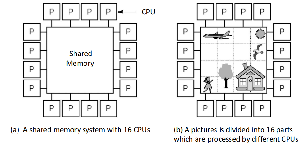
统一地址空间不等于物理上只有一个 memory。共享地址空间可由物理共享 memory 实现，也可由分布式 memory 加硬件/软件支持实现。

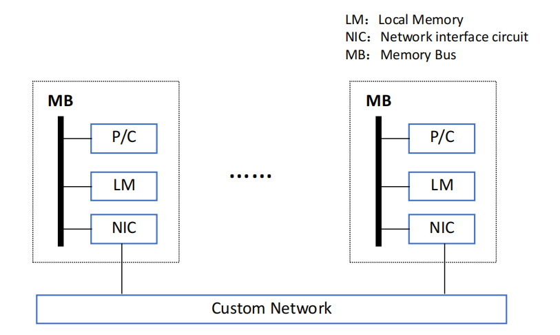
Multi-computer system based on message passing

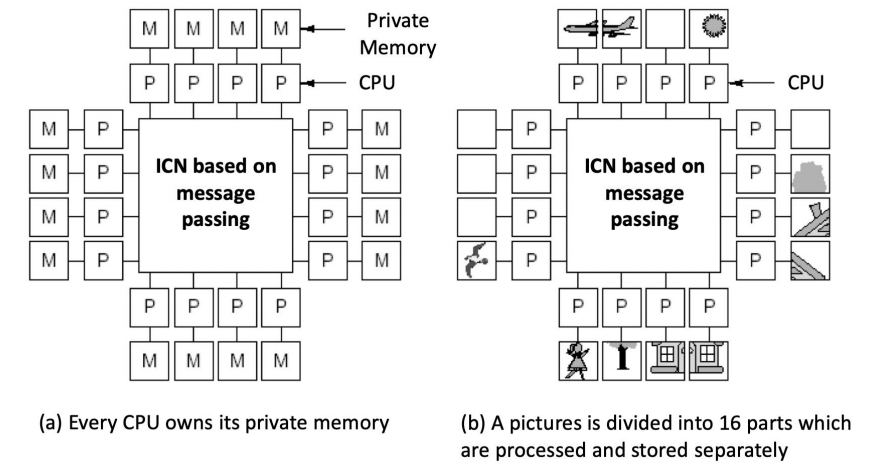
Multi-computer system 中，若处理器 A 需要把数据发给处理器 B，A 必须以 message 形式发送。

NORMA (No-Remote Memory Access)

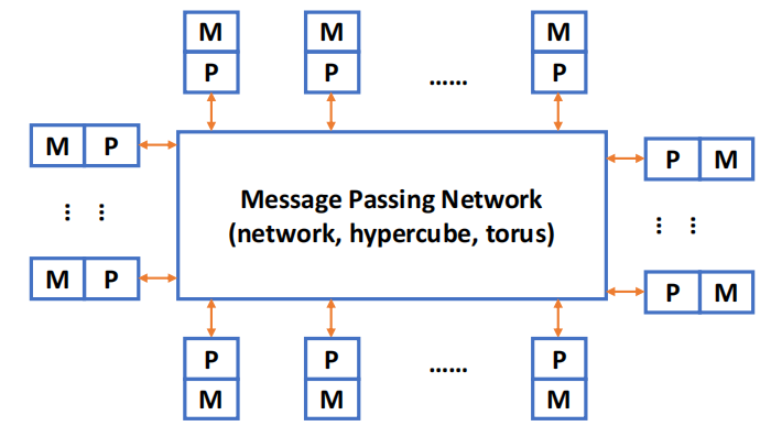
每个节点只能直接访问自己的 local memory，节点间通过 message passing network 通信。

5. 2 Shared-Memory MIMD Models¶

模型	全称	特点
UMA	Uniform Memory Access	所有处理器访问任意 memory word 的时间相同
NUMA	Non-Uniform Memory Access	所有 CPU 共享统一地址空间，但访问 remote memory 慢于 local memory
COMA	Cache Only Memory Access	NUMA 的特殊情况，所有 caches 形成统一地址空间

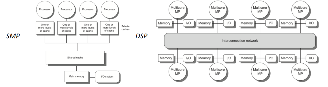
① UMA¶

UMA 又称 SMP（symmetric shared-memory multiprocessors） 或 centralized shared-memory multiprocessors。

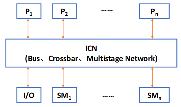
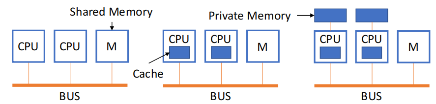
physical memory 被所有 processors 均匀共享
所有 processors 访问任意 memory word 所需时间相同
每个 processor 可以配备 private cache 或 private memory

② NUMA¶

NUMA 又称 distributed shared-memory multiprocessor。

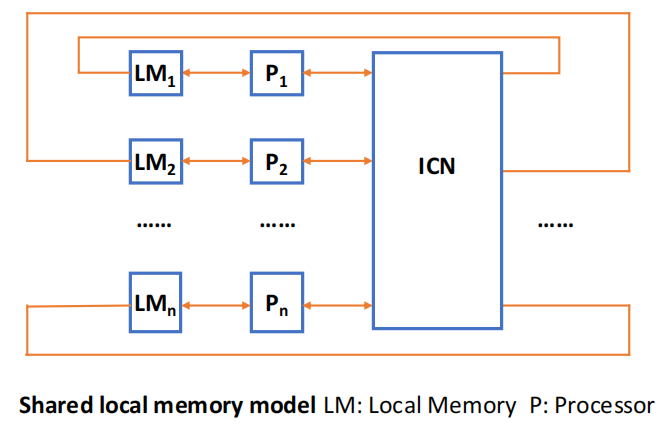
所有 CPU 共享统一 address space
使用 LOAD / STORE 指令访问 remote memory
remote memory access 慢于 local memory access
NUMA processor 可以使用 cache

NUMA 类型	含义
NC-NUMA	Non Cache NUMA，没有 cache，remote memory latency 不被 cache 隐藏
CC-NUMA	Coherent Cache NUMA，使用 cache，并维护 cache coherence

UMA and NUMA

③ COMA¶

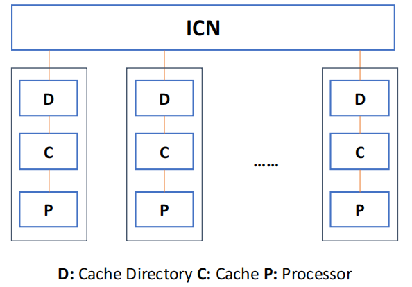
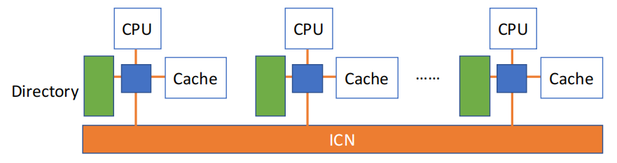
COMA 是 NUMA 的特殊情况。每个 processor node 没有传统存储层次，所有 caches 形成统一地址空间。系统使用 distributed cache directory 进行 remote cache access，数据初始可任意分配，运行时会迁移到实际使用位置。

5. 3 Further division of MIMD multi-computer system¶

类型	全称	特点
MPP	Massively Parallel Processors	由数百个处理器组成的大规模并行计算机系统
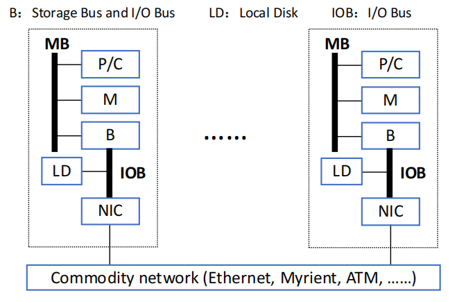
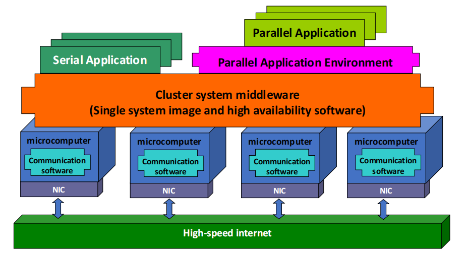
COW	Cluster of Workstations	大量 PC 或 workstations 通过商用网络连接

① MPP¶

通常使用 standard commercial CPUs
使用高性能私有 interconnection network，低延迟、高带宽传递 messages
I/O 能力强
支持专门 fault-tolerant processing
开发困难、价格高、市场有限，常被视为国家综合实力标志之一

② COW¶

可完全由 commercially available components 组装
组件量产，性价比较高
主要有 centralized 和 decentralized 两类
通常通过 Ethernet、Myrinet、ATM 等 commodity network 连接

5. 4 Challenges of Parallel Processing¶

多处理器应用范围很广，从几乎不需要通信的独立任务，到需要线程频繁通信的并行程序。并行处理的两个主要障碍：

程序可利用的 parallelism 有限。
communication cost 相对较高。

这两点都可用 Amdahl's Law 解释。

100 个处理器要达到 80 倍加速，串行比例最多多少？

Amdahl's Law：

\[ Speedup = \frac{1}{F_s + \frac{1 - F_s}{100}} \]

令 Speedup = 80：

\[ \frac{1}{80} = F_s + \frac{1 - F_s}{100} \]

解得：

\[ F_s \approx 0.0025 = 0.25\% \]

因此要用 100 个处理器达到 80 倍加速，原始计算中最多只能有约 0.25% 是串行部分。

100 处理器应用中，50 处理器阶段最多占多少？

假设 95% 时间可完美使用 100 个处理器，剩余 5% 中有 x 使用 50 个处理器，其余 0.05 - x 串行。希望加速比为 80：

\[ \frac{1}{80} = \frac{0.95}{100} + \frac{x}{50} + (0.05 - x) \]

解得：

\[ x = 0.048 \]

即剩余时间中约 4.8% 必须仍能使用 50 个处理器，只有约 0.2% 能串行。

Remote communication 的 CPI 代价？

假设 32-processor multiprocessor 中 remote memory reference 延迟 100 ns，processor clock rate 4 GHz，base CPI 为 0.5，有 0.2% 指令涉及 remote communication reference。

cycle time：

\[ \frac{1}{4GHz}=0.25ns \]

remote request cost：

\[ \frac{100ns}{0.25ns}=400 \text{ cycles} \]

CPI：

\[ CPI = 0.5 + 0.2\% \times 400 = 1.3 \]

若没有 communication，CPI 为 0.5，因此无通信版本快：

\[ \frac{1.3}{0.5}=2.6 \]

6 Cache Coherence¶

6. 1 Basic Concepts¶

Shared-memory multiprocessor 中，每个 core 往往有自己的 cache。同一 memory block 可能在多个 cache 中存在副本，若某个 processor 修改了自己的副本，其它副本可能过期，这就是 cache coherence problem。

Cache coherence protocol 是由 cache、CPU 和 memory 共同实现的一组规则，用来防止多个 caches 中出现同一数据的不同版本。

概念	含义	需要
Memory Consistency	写入值什么时候会被读到；不同地址访问之间的可见顺序	Memory consistency model
Cache Coherence	同一地址的多个 cache 副本如何保持一致	Cache coherence protocol

Cache coherence 要求：

任意 processor 的 read 都应返回该地址最近写入的值
对同一地址的多个 writes，所有 processors 必须看到相同顺序
正确 coherence 应让程序员无法通过 load/store 结果判断系统是否有 cache 或 cache 在哪里

机制	含义	好处
Migration	数据项可移动到 local cache 中透明使用	降低 remote shared data 访问延迟，减少 shared memory bandwidth demand
Replication	多个 processor 同时读共享数据时，在 local cache 中复制副本	降低读共享数据的访问延迟和争用

系统	协议	做法
UMA	Snoopy coherence protocols	所有 processors 监听 bus；某 processor 修改 private cache 中数据时，在 bus 上广播 invalidate 或 update
NUMA	Directory protocol	directory 记录哪些 processors 缓存了某个 block；写 shared block 时按 directory 点对点发送 invalidation

写策略	含义
Write-through	写 cache line 时同时修改 memory，memory 始终保持最新
Write-back	写操作不直接写 memory，而是把 cache line 标记为 dirty；memory 可能过期，之后再 write back

Write-through cache coherency protocol 中，local / remote 操作大致如下：

操作	Local Request	Remote Request
Read Miss	从 memory 取数据
Read Hit	使用 local cache data
Write Miss	修改 memory
Write Hit	修改 cache 和 memory	使对应 cache item invalid

Write-through 基本协议可变化的点：

remote write hit 时使用 update strategy 还是 invalidate strategy
write miss 时是否把对应 word 装入 cache，即是否使用 write-allocate policy

协议	做法
Write invalidate protocol	某 processor 写入时，使其它 cache 中该 block 的副本失效
Write update / write broadcast protocol	某 processor 写入时，更新所有 cache 中该数据项的副本

Write invalidate 在 snooping bus 上常与 write-back cache 结合使用。

6. 2 MSI Protocol¶

MSI 是 basic write invalidation snooping protocol，包含 3 种 block states：

状态	含义
Invalid (I)	cache item 中数据无效
Shared (S)	private cache 中该 block 可能被多个 cache 共享，memory 中值是最新的
Modified (M)	该 block 已在 private cache 中更新，memory 中值过期；同时隐含该副本是 exclusive 的

MSI protocol 操作示例

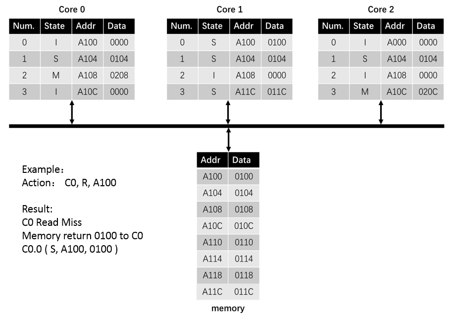
每个 core 有 4-line direct-mapped write-back cache，使用 basic write invalidation snooping protocol。

操作 1：C0, R, A10C
答案
- C0 read miss
- C2 write back A10C
- Memory A10C: 010C -> 020C
- C2.3 变为 (S, A10C, 020C)
- memory 返回 020C 给 C0
- C0.3 变为 (S, A10C, 020C)
操作 2：C1, W, A104, 0204
答案
- C1 write hit
- invalidates C0 和 C2 中 A104 的副本
- C0.1 变为 (I, A104, 0104)
- C2.1 变为 (I, A104, 0104)
- C1.1 变为 (M, A104, 0204)
操作 3：C0, W, A118, 0308
答案
- C0 write miss
- C0 write back A108
- Memory A108: 0108 -> 0208
- memory 返回 0118 给 C0
- C0.2 先变为 (M, A118, 0118)
- 写入后 C0.2 变为 (M, A118, 0308)

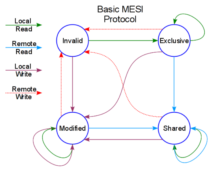
6. 3 MESI and MOESI¶

MESI 在 MSI 基础上增加 Exclusive 状态：

状态	含义
Invalid	cache item 中数据无效
Shared	多个 cache 可能有该行副本，memory 中值最新
Exclusive	没有其它 cache 持有该行副本，memory 中值最新
Modified	本 cache 数据有效且被修改，memory 过期，没有其它 cache 副本

若 block 只在单个 cache 中且 clean，该 cache 写入时可从 Exclusive -> Modified，无需在 bus 上广播。

MESI protocol state transition rules

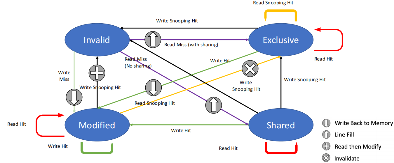
MESI protocol working process

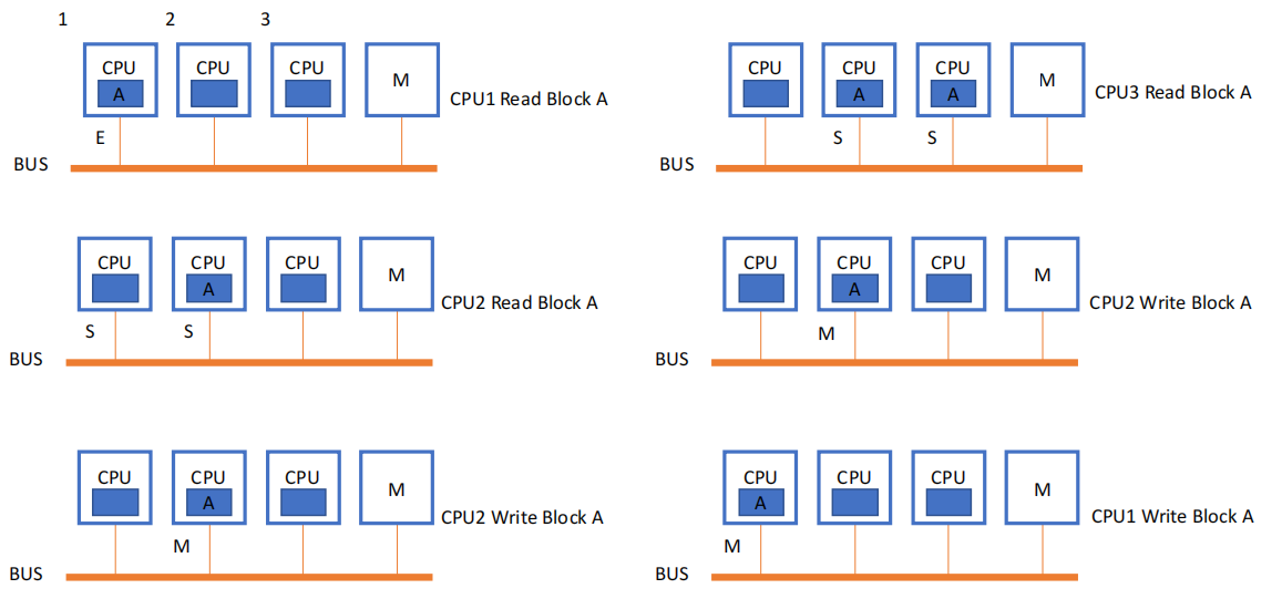
MOESI 在 MESI 基础上增加 Owned 状态：表示该 cache 拥有该 block，memory 中值过期。它允许 Modified -> Owned，不必先把 shared block 写回 memory。

6. 4 Directory Protocol¶

Directory-based protocol 常用于 distributed-memory / NUMA multiprocessor。每个节点增加 directory，用来记录每个可能被缓存 block 的状态。

Directory 中维护的信息包括：

哪些 caches 有该 block 的副本
该 block 是否 dirty
owner node ID 或 sharer set

每个 block 的 directory states：

状态	含义
Invalid / uncached	没有节点缓存该 block
Shared	一个或多个节点缓存该 block，memory 中值最新，directory 记录 node ID set
Modified / exclusive	恰好一个节点有该 block，memory 中值过期，directory 记录 owner node ID

Directory 维护 block states 并发送 invalidation messages。

当前状态	请求	行为
Uncached	Read miss	给请求节点发送数据；请求节点成为唯一 sharer；block 变为 shared
Uncached	Write miss	给请求节点发送数据；请求节点成为 owner；block 变为 exclusive
Shared	Read miss	从 memory 给请求节点发送数据；把请求节点加入 sharing set
Shared	Write miss	给请求节点发送值；向 sharing set 中所有节点发 invalidation；sharing set 只保留请求节点；block 变为 exclusive
Exclusive	Read miss	向 owner 发送 data fetch；block 变为 shared；owner 把数据发给 directory 并写回 memory；sharers 包含旧 owner 和 requestor
Exclusive	Data write back	block 变为 uncached，sharer set 清空
Exclusive	Write miss	通知旧 owner invalidate 并把值发给 directory；requestor 成为新 owner；block 保持 exclusive

7 Memory Consistency¶

Memory consistency model 规定不同处理器上的读写操作以什么顺序对程序可见。它关注的是不同地址之间的访问顺序，而 cache coherence 主要关注同一地址多个副本的一致性。

典型例子：

Processor 1:        Processor 2:
A = 0               B = 0
...
A = 1               B = 1
if (B == 0) ...     if (A == 0) ...

Sequential consistency 要求执行结果等价于：

每个 processor 内部的 memory accesses 保持程序顺序
不同 processors 的 memory accesses 可以任意交错

这会降低潜在性能，因为硬件和编译器不能随意重排读写。

Relaxed consistency models 的核心思想：允许 reads 和 writes 乱序完成，但通过 synchronization operations 强制关键顺序。

用 X -> Y 表示 operation X 必须在 operation Y 完成前完成。

模型/规则	放松的顺序
Sequential consistency	要求 `R -> W`、`R -> R`、`W -> R`、`W -> W` 全部保持
Total Store Ordering (TSO)	放松 `W -> R`
Partial Store Order (PSO)	放松 `W -> W`
Weak Ordering / Release Consistency	放松 `R -> W` 和 `R -> R`，依赖同步操作恢复必要顺序

8 Domain-Specific Architectures¶

DSA（Domain-Specific Architectures） 面向特定领域抽取性能。Moore's Law 曾让通用处理器通过 deep memory hierarchy、wide SIMD units、deep pipelines、branch prediction、out-of-order execution、speculative prefetching、multithreading、multiprocessing 等机制，从不了解底层架构的软件中榨取性能。

DSA 的目标是：针对领域特征直接设计硬件和软件接口，减少通用性带来的浪费。

8. 1 DSA Guidelines¶

使用 dedicated memories，最小化 data movement
把资源投入更多 arithmetic units 或更大的 memories
使用匹配领域的最简单 parallelism 形式
把 data size 和 data type 降到领域所需的最简单形式
使用 domain-specific programming language

8. 2 CNN and TPU¶

从体系结构角度看，CNN 需要关注：

技术	作用
Batches	权重从 memory 取出后可在多个 inputs 间复用，提高 operational intensity
Quantization	使用 8-bit 或 16-bit fixed point，降低存储和计算成本
Common kernels	matrix-vector multiply、matrix-matrix multiply、ReLU、Sigmoid 等

TPU（Tensor Processing Unit） 是 Google 的 DNN ASIC：

256 × 256 8-bit matrix multiply unit
large software-managed scratchpad
作为 PCIe bus 上的 coprocessor

TPU ISA 的主要操作：

指令	作用
Read_Host_Memory	从 CPU memory 读入 unified buffer
Read_Weights	从 weight memory 读权重到 weight FIFO，作为 matrix unit 输入
MatrixMatrixMultiply / Convolve	从 unified buffer 到 accumulators 执行矩阵乘、向量矩阵乘、element-wise 乘或卷积
Activate	计算 activation function
Write_Host_Memory	把 unified buffer 中的数据写回 host memory

TPU 对 DSA guidelines 的体现：

Guideline	TPU 实现
Dedicated memories	24 MiB dedicated buffer，4 MiB accumulator buffers
投入 arithmetic units / memories	相比 server-class CPU，约 60% 资源用于 memory，算术单元约 250 倍
匹配领域的并行形式	利用 2D SIMD parallelism
降低 data size/type	主要使用 8-bit integers
Domain-specific language	使用 TensorFlow

Initial Code	Before Shuffle	After 1st Shuffle	Connected PE (1st Shuffle)	After 2nd Shuffle	Connected PE (2nd Shuffle)	After 3rd Shuffle	Connected PE (3rd Shuffle)
0	000	000	0	000	0	000	0
1	001	010	2	100	4	001	1
2	010	100	4	001	1	010	2
3	011	110	6	101	5	011	3
4	100	001	1	010	2	100	4
5	101	011	3	110	6	101	5
6	110	101	5	011	3	110	6
7	111	111	7	111	7	111	7

Initial Code	Before Shuffle	After 1st Shuffle	Connected PE (1st Shuffle)	After 2nd Shuffle	Connected PE (2nd Shuffle)	After 3rd Shuffle	Connected PE (3rd Shuffle)
0	000	000	0	000	0	000	0
1	001	010	2	100	4	001	1
2	010	100	4	001	1	010	2
3	011	110	6	101	5	011	3
4	100	001	1	010	2	100	4
5	101	011	3	110	6	101	5
6	110	101	5	011	3	110	6
7	111	111	7	111	7	111	7

Initial Code	Before Shuffle	After 1st Shuffle	Connected PE (1st Shuffle)	After 2nd Shuffle	Connected PE (2nd Shuffle)	After 3rd Shuffle	Connected PE (3rd Shuffle)
0	000	000	0	000	0	000	0
1	001	010	2	100	4	001	1
2	010	100	4	001	1	010	2
3	011	110	6	101	5	011	3
4	100	001	1	010	2	100	4
5	101	011	3	110	6	101	5
6	110	101	5	011	3	110	6
7	111	111	7	111	7	111	7