1 AVL Trees, Splay Trees and Amortized Analysis
1. 1 AVL Trees
基本性质
The inorder traversal sequence of an AVL tree must be in sorted (non-decreasing) order.
答案
AVL 树仍具有二叉搜索树的性质,故答案为 \(\textnormal{T}\)
平衡因子 \(BF(node) = h_L -h_R\)
温馨提示
- 完美二叉树:全满,所有层无空缺,叶子在同一层
- 完全二叉树:前满后左齐,最后一层可不满,但必须左连续
An AVL tree with the balance factors of all the non-leaf nodes being 0 must be a perfect binary tree.
答案
\(\textnormal{T}\)
For an AVL tree, the balance factors of all the non-leaf nodes are 0 if the tree is a complete binary tree.
答案
\(\textnormal{F}\)
时间复杂度
For the Turnpike reconstruction algorithm of \(N\) points, assuming that the distance set \(D\) is maintained as an AVL tree, the running time is \(O(N^2\log{N})\) if no backtracking happens.
答案
AVL 树每次查找和删除操作的时间复杂度为 \(O(\log |D|)\)。添加第 \(k\) 个点时,若无回溯,对于已确定的 \(k-1\) 个点,需要查找该点与候选点的距离是否在 D 中,若存在则从 \(D\) 中删除,耗时 \(O(k \log N)\),则总耗时为 \(O(\sum\limits_{k=2}^{N} k \log N) = O(N^2 \log N)\),答案为 \(\textnormal{T}\)
AVL 树的查找
Which one of the following is NOT true about B+ trees and AVL trees: they are both \(\underline{\qquad}\) .
\(\textnormal{A}\). balanced binary trees \(\qquad\) \(\textnormal{B}\). fit for sequential searches
\(\textnormal{C}\). fit for random searches \(\qquad\) \(\textnormal{D}\). fit for range searches
答案
AVL 树是二叉搜索树,无有序链接结构,顺序查找需逐个遍历节点,效率 \(O (n)\),不适合顺序查找,故答案为 \(\textnormal{B}\)
AVL 树的插入和删除
Delete a node \(v\) from an AVL tree \(T_ 1\), we can obtain another AVL tree \(T_ 2\). Then insert \(v\) into \(T_ 2\), we can obtain another AVL tree \(T_ 3\). Which one(s) of the following statements about \(T_ 1\) and \(T_ 3\) is(are) true?
- I、If \(v\) is a leaf node in \(T_ 1\), then \(T_ 1\) and \(T_ 3\) might be different.
- II、If \(v\) is not a leaf node in \(T_ 1\), then \(T_ 1\) and \(T_ 3\) must be different.
- III、If \(v\) is not a leaf node in \(T_ 1\), then \(T_ 1\) and \(T_ 3\) must be the same.
\(\textnormal{A}. \,\) I only \(\qquad\) \(\textnormal{B}. \,\) II only \(\qquad\) \(\textnormal{C}. \,\) I and II only \(\qquad\) \(\textnormal{D}. \,\) I and III only
答案
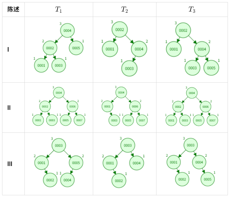
故答案为 \(\textnormal{A}\)
1. 2 Splay Trees
基本性质
All of the Zig, Zig-zig, and Zig-zag rotations not only move the accessed node to the root, but also roughly half the depth of most nodes on the path.
答案
\(\textnormal{T}\)
All of the Zig, Zig-zig, and Zig-zag rotations in a splay tree not only move the accessed node to the root, but also roughly half the depth of most nodes in the tree.
答案
\(\textnormal{F}\)
Splay 树的查找
In a splay tree, if we only have to find a node without any more operation, it is acceptable that we don't push it to root and hence reduce the operation cost. Otherwise, we must push this node to the root position.
答案
根据伸展树的定义,每一次访问操作(查找、插入、删除)都需要将被访问的节点伸展到根(即使是单次查找操作也必须执行伸展),故答案为 \(\textnormal{F}\)
In a splay tree, for any non-root node X, its parent P and grandparent G (guranteed to exist), the correct operation to splay X to G is to rotate X upward twice.
答案
将非根节点 \(X\) 伸展到祖父 \(G\) 时,需根据 \(X\)、父节点 \(P\)、祖父 \(G\) 的结构,执行 zig-zig 或 zig-zag 旋转,而非简单的将 \(X\) 向上旋转两次,故答案为 \(\textnormal{F}\)
Splay 树的删除
After deleting 7 from the given splay tree, which of the following statements about the resulting tree is impossible?
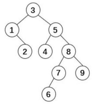
\(\textnormal{A}\). 8 is the root \(\qquad\) \(\textnormal{B}\). 1 and 4 are siblings \(\qquad\)\(\textnormal{C}\). 6 is the root \(\qquad\) \(\textnormal{D}\). 6 is the grandparent of 5
答案
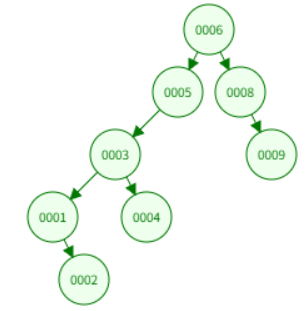
答案为 \(\textnormal{D}\),伸展树删除操作后结果如下:
时间复杂度
Start from \(N\) single-node splay trees, let's merge them into one splay tree in the following way: each time we select two splay trees, delete nodes one by one from the smaller tree and insert them into the larger tree. Then which of the following statements is NOT true?
\(\textnormal{A}\). In any sequence of \(N-1\) merges, there are at most \(O(N\log N)\) inserts.
\(\textnormal{B}\). Any node can be inserted at most \(\log N\) times.
\(\textnormal{C}\). The amortized time bound for each insertion is \(O(\log ^2 N)\).
\(\textnormal{D}\). The amortized time bound for each merge is \(O(\log N)\).
答案
每个节点仅当所在树是较小树时才会被插入到另一棵树中,插入后,节点所在树的大小至少翻倍,每个节点最多插入 \(logN\) 次,总插入次数为 \(O(N\log N)\),故 \(\textnormal{A}\) 、\(\textnormal{B}\) 选项正确
向大小为 \(m\) 的 Splay 树插入一个节点,均摊时间复杂度为 \(O(\log m)\),故单个节点的总插入时间为 \(O(\log N \times \log N)\),均摊插入时间为 \(\frac{O(N \log^2 N)}{O(N \log N)} = O(\log N)\),由于 \(O\) 表示上界,\(O(\log N)\) 是 \(O(\log^2 N)\) 的子集,故 \(\textnormal{C}\) 选项正确
同理,均摊合并时间为 \(\frac{O(N \log^2 N)}{O(N)} = O(\log^2 N)\),故 \(\textnormal{D}\) 选项错误,答案为 \(\textnormal{D}\)
1. 3 AVL Trees V.S. Splay Trees
自调整结构
In typical applications of data structures, it is not a single operation that is performed, but rather a sequence of operations, and the relevant complexity measure is not the time taken by one operation but the total time of a sequence. Hence instead of imposing any explicit structural constraint, we allow the data structure to be in an arbitrary state, and we design the access and update algorithms to adjust the structure in a simple, uniform way, so that the efficiency of future operations is improved. We call such a data structure self- adjusting. For example skew heaps and splay trees are such kind of structures.
Which one of the following statements is FALSE about self-adjusting data structures?
\(\textnormal{A}\). They need less space, since no balance information is kept.
\(\textnormal{B}\). Their access and update algorithms are easy to understand and to implement.
\(\textnormal{C}\). In an amortized sense, ignoring constant factors, they can be at least as efficient as balanced structures.
\(\textnormal{D}\). Less local adjustments take place than in the corresponding balanced structures, especially during accesses.
答案
自调整结构(如伸展树)在访问操作时会执行伸展操作(包含多次旋转调整);而平衡结构(如AVL树)的访问操作不需要任何调整。因此,自调整结构在访问时的局部调整更多,而非更少,答案为 \(\textnormal{D}\)
1. 4 Amortized Analysis
基本概念
In amortized analysis, a good potential function should always assume its minimum at the start of the sequence.
答案
\(\textnormal{T}\)
Amortized analysis is a technique to provide an upper bound on the actual cost of a sequence of operations
答案
\(\textnormal{T}\)
势能函数的缩放性质
If \(\Phi\) is a potential function associated with a data structure \(S\), then \(3\Phi\) is also a potential function that can be associated with \(S\). Moreover, the amortized running time of each operation with respect to \(3\Phi\) is at most triple the amortized running time of the operation with respect to \(\Phi\).
答案
\(\hat{A}_i = c_i + (\Phi_i - \Phi_{i-1})\),\(\hat{A}'_i = c_i + (3\Phi_i - 3\Phi_{i-1}) = 3\hat{A}_i - 2c_i \leq 3\hat{A}_i\),故答案为 \(\textnormal{T}\)
Suppose we have a potential function \(\Phi\) such that for all \(\Phi(D_i) \geq \Phi(D_0)\) for all \(i\), but \(\Phi(D_0) \neq 0\). Then there exists a potential \(\Phi'\) such that \(\Phi'(D_0) = 0, \Phi'(D_i) \geq 0\) for all \(i \geq 1\), and the amortized costs using \(\Phi'\) are the same as the amortized costs using \(\Phi\).
答案
令 \(\Phi'(D) = \Phi(D) - \Phi(D_0)\),则 \(\hat{c}_i' = c_i + \Phi'(D_i) - \Phi'(D_{i-1}) = c_i + \Phi(D_i) - \Phi(D_{i-1}) = \hat{c}_i\),故答案为 \(\textnormal{T}\)
worst-case bound \(≥\) amortized-case bound \(≥\) average-case bound
Amortized bounds are weaker than the corresponding worst-case bounds, because there is no guarantee for any single operation.
答案
\(\textnormal{T}\)
For one operation, if its amortized time bound is \(O(logN)\), then its worst-case time bound must be \(O(logN)\).
答案
\(\textnormal{F}\)
For one operation, if its worst-case time bound is \(O(logN)\), then its amortized time bound must be \(O(logN)\).
答案
\(\textnormal{T}\)
For one operation, if its average time bound is \(O(logN)\), then its amortized time bound must be \(O(logN)\).
答案
\(\textnormal{F}\)
Recall the amortized analysis for Splay Tree and Leftist Heap, from which we can conclude that the amortized cost (time) is never less than the average cost (time).
答案
\(\textnormal{F}\)
简单的摊还分析
A queue can be implemented by using two stacks \(SA\) and \(SB\) as follows:
- To enqueue x, we push x onto \(SA\).
- To dequeue from the queue, we pop and return the top item from \(SB\). However, if \(SB\) is empty, we first fill it (and empty \(SA\)) by popping the top item from \(SA\), pushing this item onto \(SB\), and repeat until \(SA\) is empty.
Assuming that push and pop operations take \(O(1)\) worst-case time, please select a potential function \(\Phi\) which can help us prove that enqueue and dequeue operations take \(O(1)\) amortized time (when starting from an empty queue).
\(\textnormal{A}\). \(\Phi=2\ |\ SA\ |\) \(\qquad\) \(\textnormal{B}\). \(\Phi= |\ SA\ |\) \(\qquad\) \(\textnormal{C}\). \(\Phi=2\ |\ SB\ |\) \(\qquad\) \(\textnormal{D}\). \(\Phi= |\ SB\ |\)
答案
考虑 \(\text{SB}\) 为空时的出栈操作,要求势能大幅下降,排除 \(\textnormal{C}\) 和 \(\textnormal{D}\)
考虑 \(\textnormal{A}\) 和 \(\textnormal{B},\)实际成本 \(c_i = 2 |\text{SA}| + 1\),均摊成本分析如下:
| 势能函数 | \(\Phi_{\text{before}}\) | \(\Phi_{\text{after}}\) | \(\Delta \Phi\) | 均摊成本 \(a_i\) |
|---|---|---|---|---|
| \(\Phi= 2 \lvert \text{SA} \rvert\) | \(2k\) | \(0\) | \(-2k\) | \(1\) |
| \(\Phi= \lvert \text{SA} \rvert\) | \(k\) | \(0\) | \(-k\) | \(k + 1\) |
综上,正确答案为 \(\textnormal{A}\)
In this problem, we would like to find the amortized cost of insertion in a dynamic table \(T\). Initially the size of the table \(T\) is \(1\). The cost of insertion is \(1\) if the table is not full. When an item is inserted into a full table, the table \(T\) is expanded as a new table of size \(5\) times larger. Then, we copy all the elements of the old table into this new table, and insert the item in the new table.
Let \(num(T)\) be the number of elements in the table \(T\), and \(size(T)\) be the total number of slots of the table. Let \(D_i\) denote the table after applying the \(i\) th operation on \(D_{i-1}\).
Which of the following potential function \(\Phi(D_i)\) can help us achieve \(O(1)\) amortized cost per insertion?
\(\textnormal{A}\). \(\Phi(D_i) = num(T) - \frac{size(T)}{5}\) \(\qquad\) \(\qquad\) \(\textnormal{B}\). \(\Phi(D_i) = num(T) + \frac{size(T)}{5}\)
\(\textnormal{C}\). \(\Phi(D_i) = \frac{5}{4}\left(num(T) - \frac{size(T)}{5}\right)\) \(\qquad\) \(\textnormal{D}\). \(\Phi(D_i) = \frac{5}{4}\left(num(T) + \frac{size(T)}{5}\right)\)
答案
高成本操作需要势能的大幅下降来抵消实际 cost,故排除 \(\textnormal{B}\) 和 \(\textnormal{D}\)
若插入时表不满,则实际成本 \(c_i = 1\),插入后 \(\text{size}\) 不变;若插入时表满,则实际成本 \(c_i = 1 + s\),插入后 \(\text{size} =5s\),而 \(a_i = c_i + (\Phi_2 - \Phi_1)\)
对于选项 \(\textnormal{A}\),分析如下:
| \(\Phi(D_i) = num(T) - \frac{size(T)}{5}\) | 表不满 | 表满 |
|---|---|---|
| 初始势能 \(\Phi_1\) | \(num - \frac{size}{5}\) | \(s - \frac{s}{5} = \frac{4s}{5}\) |
| 最终势能 \(\Phi_2\) | \((num+1) - \frac{size}{5}\) | \((s+1) - \frac{5s}{5} = 1\) |
| 势能变化 \(\Delta\Phi\) | \(1\) | \(1 - \frac{4s}{5}\) |
| 均摊成本 \(a_i\) | \(1 + 1 = 2\) | \(2 + \frac{s}{5}\) |
对于选项 \(\textnormal{C}\),分析如下:
| \(\Phi(D_i) = \frac{5}{4}\left(num(T) - \frac{size(T)}{5}\right)\) | 表不满 | 表满 |
|---|---|---|
| 初始势能 \(\Phi_1\) | \(\frac{5}{4}num - \frac{size}{4}\) | \(\frac{5}{4}s - \frac{s}{4} = s\) |
| 最终势能 \(\Phi_2\) | \(\frac{5}{4}(num+1) - \frac{size}{4}\) | \(\frac{5}{4}(s+1) - \frac{5s}{4} = \frac{5}{4}\) |
| 势能变化 \(\Delta\Phi\) | \(\frac{5}{4}\) | \(\frac{5}{4} - s\) |
| 均摊成本 \(a_i\) | \(\frac{9}{4}\) | \(\frac{9}{4}\) |
综上,只有 \(\Phi(D_i) = \frac{5}{4}\left(num(T) - \frac{size(T)}{5}\right)\) 能使两次插入场景的均摊成本均为常数,故正确答案为 \(\textnormal{C}\)
A \(n\)-nodes AVL tree \(T\) performs insertion or deletion in the worst case that costs \(a_0 \lg n + b_0\), \(a_1 \lg n + b_1\), respectively, where \(a_0, a_1, b_0, b_1\) are constants. Now, we start from an empty tree, perform a sequence of \(n\) insertions or deletions in the AVL tree. To analysis the amortized cost per insertion or deletion, we define a potential function \(\Phi(T) = a_1 \sum_{i=1}^{n} \lg i\). What is the amortized cost per insertion or deletion?
\(\textnormal{A}\). \(O(\lg n )\) for insertion \(O(\lg n)\) for deletion \(\qquad\) \(\textnormal{B}\). \(O(\lg n )\) for insertion \(O(1)\) for deletion
\(\textnormal{C}\). \(O(1)\) for insertion, \(O(\lg n)\) for deletion \(\qquad\) \(\textnormal{D}\). \(O(1)\) for insertion, \(O(1)\) for deletion
答案
\(\hat{c}_{\text{insert}} = c_{\text{insert}} + \Delta\Phi = (a_0 \lg k + b_0) + a_1 \lg(k+1) = O(\lg n)\)
\(\hat{c}_{\text{delete}} = c_{\text{delete}} + \Delta\Phi = (a_1 \lg k + b_1) - a_1 \lg k = b_1 = O(1)\)
故正确答案为 \(\textnormal{B}\)
二进制计数器递增成本计算
We have a binary counter of k bits. Each time we conduct an increment on the counter: \(X = X + 1 (\text{mod } 2^k)\) and the cost of the increment is the number of bits we need to flip. For example, when \(k = 3\), currently we have \(X = 010\), after increment we have \(X = 011\). Then this increment costs 1 because only 1 bit flips after increment. If we conduct the increment again, \(X = 100\). Then this increment costs 3 because we flip 3 bits. Now we conduct n consecutive increments and estimate the total cost. Which of the following statements are TRUE?
- If the initial value of the counter is 0, the total cost is \(O(n)\)
- If the initial value of the counter is 0, the total cost is \(O(n \log k)\)
- If \(n = \Omega(k)\), the total cost is \(O(n)\)
- If \(n = \Omega(k)\), the total cost is \(O(n \log k)\)
答案
对于二进制计数器的第 \(i\) 位,每 \(2^{i-1}\) 次递增翻转 1 次
当初始值为 0 时,总成本 \(= \sum\limits_{i=1}^k \left\lfloor \frac{n}{2^{i-1}} \right\rfloor \leq n \cdot \sum\limits_{j=0}^\infty \frac{1}{2^j} = 2n = O(n)\)
当 \(n=\Omega(k)\),即 \(n\) 至少是 \(k\) 的常数倍时,总成本不受 \(k\) 的影响,总成本 \(= O(n)\)
综上,答案为 1 和 3
Minimum Degree Spanning Tree
Consider the Minimum Degree Spanning Tree problem: Given a connected undirected graph \(G(V, E)\), find a spanning tree \(T\) whose maximum degree over its vertices is minimized over all spanning trees of \(G\). The problem can be shown to be NP-hard by reduction from the Hamiltonian Path Problem. On the other hand, we can use local search to design approximating algorithms. Denote \(d(u)\) as the degree of vertex \(u\) on a tree \(T\). Consider the following algorithm:
- Find an arbitrary spanning tree \(T\) of \(G\).
- If there's some edge \(e \in E(G) \setminus E(T)\) with endpoints \(u, v\), and there's some other vertex \(w\) on the path between \(u, v\) on \(T\) such that \(\max\{d(u), d(v)\} + 1 < d(w)\), then we replace an edge \(e'\) incident to \(w\) on \(T\) with \(e\), i.e. \(T := T \cup \{e\} \setminus \{e'\}\).
- Repeat Step (2) until there's no edge to replace.
It can be shown that this algorithm will terminate at a solution with maximum vertex degree \(OPT + O(\log |V|)\). To show the algorithm will terminate in finite steps, a useful technique is to define a nonnegative potential function \(\Phi(T)\) and to show \(\Phi(T)\) is strictly decreasing after each step. Which of the following potential functions below satisfies the above requirements?
\(\textnormal{A}\). \(\Phi(T) = \sum_{v \in V} d(v)\) \(\qquad\) \(\qquad\) \(\qquad\) \(\textnormal{B}\). \(\Phi(T) = \sum_{(u,v) \in E(T)} \max\{d(u), d(v)\}\)
\(\textnormal{C}\). \(\Phi(T) = \sum_{u \in V} \sum_{v \in V, v \neq u} \sum_{w \in V, w \neq u, v} \max\{d(u), d(v), d(w)\}\) \(\qquad\) \(\textnormal{D}\). \(\Phi(T) = \sum_{v \in V} 3^{d(v)}\)
答案
算法的边替换规则:选非树边 \(e=(u,v)\),在 \(T\) 中 \(u-v\) 路径上找顶点 \(w\) 满足 \(\max\{d(u),d(v)\}+1 < d(w)\),替换 \(w\) 关联的边 \(e'\)
对于 \(\Phi(T) = \sum_{v \in V} d(v)\),生成树的总度数是固定的:树有 \(|V|-1\) 条边,每条边贡献 \(2\) 度,总度数为 \(2(|V|-1)\)。无论如何替换边,生成树的边数不变,因此总度数不变,\(\Phi(T)\) 不会递减,排除 \(\textnormal{A}\)
对于 \(\Phi(T) = \sum_{(u,v) \in E(T)} \max\{d(u),d(v)\}\),替换边后,\(u\) 和 \(v\) 的度数会增加,与 \(u\)、\(v\) 关联的其他边的 \(\max\{d(\cdot),d(\cdot)\}\) 项可能增大,\(\Phi(T)\) 可能不递减,排除 \(\textnormal{B}\)
对于 \(\Phi(T) = \sum_{u \in V} \sum_{v \in V, v \neq u} \sum_{w \in V, w \neq u,v} \max\{d(u),d(v),d(w)\}\),三重求和形式过于复杂,且无法通过算法的边替换规则保证其严格递减,排除 \(\textnormal{C}\)
对于 \(\Phi(T) = \sum_{v \in V} 3^{d(v)}\),替换后,\(d'(u)=d(u)+1\)、\(d'(v)=d(v)+1\)、\(d'(w)=d(w)-1\),其他顶点度数不变,则:
由 \(\max\{d(u),d(v)\}+1 < d(w)\) 得 \(d(u) \leq \max\{d(u),d(v)\} < d(w)-1\),同理有 \(d(v) < d(w)-1\),则 \(3^{d(u)} \leq 3^{d(w)-2}\),\(3^{d(v)} \leq 3^{d(w)-2}\)
进而 \(3^{d(u)} + 3^{d(v)} \leq 2 \cdot 3^{d(w)-2} < 3^{d(w)-1}\),\(\Phi(T') < \Phi(T)\),即 \(\Phi(T)\) 严格递减
综上所述,答案为 \(\textnormal{D}\)
斐波那契堆的势能函数
Which one of the following statements is FALSE?
\(\textnormal{A}\). For red-black trees, the total time for \(m\) consecutive insertions in a tree of \(n\) nodes is \(O(n + m)\).
\(\textnormal{B}\). To obtain \(O(1)\) amortized time for the function decrease-key, the potential function used for Fibonacci heaps is \(\Phi(H) = t(H) + m(H)\), where \(t(H)\) is the number of trees in the root list of heap \(H\), and \(m(H)\) is the number of marked nodes in \(H\).
\(\textnormal{C}\). Let \(S(x)\) be the number of descendants of \(x\) (\(x\) included). If the potential function used for splay tree is \(\Phi(T) = \sum_{x \in T} \log S(x)\), then the amortized cost of one splay operation is \(O(\log n)\).
\(\textnormal{D}\). In the potential method, the amortized cost of an operation is equal to the actual cost plus the increase in potential due to this operation.
答案
在斐波那契堆中,为了确保 decrease-key 操作的摊还时间复杂度为 \(O(1)\),使用的势函数应为 \(Φ(H) = t(H) + 2m(H)\),其中 \(t(H)\) 是根列表中树的数量,\(m(H)\) 是标记节点的数量,答案为 \(\textnormal{B}\)
堆操作的摊还复杂度
Recall that the worst-case time complexities of insertions and deletions in a heap of size \(N\) are both \(O(\log N)\). Then, without changing the data structure, the amortized time complexity of insertions in a heap is also \(O(\log N)\), and that of deletions is \(O(1)\).
答案
答案是 \(\textnormal{T}\),出自王灿 2024 期中,看不懂!